Title
题目
Submillimeter diffusion MRI using an in-plane segmented 3D multi-slab acquisition and denoiser-regularized reconstruction
基于面内分段3D多块采集与去噪器正则化重建的亚毫米扩散磁共振成像
01
文献速递介绍
高分辨率扩散磁共振成像(dMRI)为白质连接的详细研究提供了强大工具。亚毫米级扩散磁共振成像(dMRI)的优势已在尸检研究中得到证实(Foxley等人,2014;Miller等人,2011;Roebroeck等人,2019)——与传统分辨率(如2毫米)相比,它能更精准地描绘弯曲和交叉的白质通路(如脑桥横纤维)。此外,亚毫米级扩散磁共振成像(dMRI)或许有助于解决扩散磁共振成像(dMRI)纤维追踪(纤维束成像)中一个已知难题,即“脑回偏差”:追踪到的纤维往往终止于脑回顶部,而非准确捕捉到向脑回壁的急转(Fritz等人,2019;Reveley等人,2015;Schilling等人,2018;Sotiropoulos和Zalesky,2019;Van Essen等人,2014)。更高的空间分辨率还有利于识别短皮质联合纤维(Song等人,2014),这类纤维通常被称为U型纤维,负责连接相邻脑回之间的皮质区域(Schmahmann和Pandya,2009)。U型纤维在研究大脑发育、功能及病理机制方面具有特殊重要性(d’Albis等人,2018;Van Dyken等人,2024)。此外,尸检研究表明(Roebroeck等人,2019),高分辨率扩散磁共振成像(dMRI)在精准描绘体积小但至关重要的皮质下结构方面极具潜力,包括详细呈现视交叉(Wedeen等人,2008)、小脑叶片(Dell’Acqua等人,2013;Wedeen等人,2008)和脑干(Aggarwal等人,2013;Tendler等人,2022;Wedeen等人,2008)等区域的交叉纤维,以及在深部脑刺激中精准定位电极靶点(Calabrese等人,2015)。 然而,要在体(in-vivo)发挥高分辨率扩散磁共振成像(dMRI)的这些优势,需克服诸多挑战。传统二维单次激发回波平面成像(2D ss-EPI)是科研与临床实践中扩散磁共振成像(dMRI)的标准采集方法,其成像机制与高空间分辨率的要求存在本质冲突(Wu和Miller,2017)。一个主要障碍是体素尺寸较小时固有的低信噪比(SNR)。在二维单次激发回波平面成像(2D ss-EPI)中,获取更多相位编码线需要更长的回波时间(TE)(导致信号强度降低),而采集更多切片需要更长的重复时间(TR)(导致扫描效率下降),这进一步加剧了信噪比(SNR)的限制。此外,为编码更高分辨率图像而进行的协议调整会影响体素定义,与高分辨率成像的目标相悖。首先,在读出方向上,提高分辨率需要更长的回波间隔,进而导致图像畸变和T2模糊加剧;其次,薄切片的激发受最大梯度强度限制,可能导致切片轮廓失真(Bernstein等人,2004)。 已有研究提出先进的采集策略以缓解二维单次激发回波平面成像(2D ss-EPI)中的这些挑战。面内加速技术可缩短回波时间(减少信号衰减)、读出时间(减少模糊)和有效回波间隔(减少畸变),但代价是欠采样重建会引入更多噪声(Griswold等人,2002;Pruessmann等人,1999)。同步多切片成像(SMS)(Feinberg和Setsompop,2013;Moeller等人,2010;Setsompop等人,2012)通过多波段激发减少重复时间(TR)并提高信噪比(SNR)效率,但需权衡噪声水平升高和射频能量沉积增加的问题。将面内加速与同步多切片成像(SMS)相结合可进一步提升扫描效率,但可达的加速因子受固有信噪比(SNR)损失和g因子惩罚的限制。近年来,基于超分辨率的方法被提出,有望实现亚毫米级扩散磁共振成像(dMRI)。gSlider技术采用二维采集方式,通过不同的射频脉冲多次激发一个薄块,从而从该块中解析出少数(约5个)薄切片(Jun等人,2024;Liao等人,2021、2023;Setsompop等人,2018)。与同步多切片成像(SMS)结合后,gSlider-SMS可有效缩短重复时间(TR)并提高信噪比(SNR)效率。近期研究提出通过采集多个具有旋转视野(FOV)的厚切片容积并结合超分辨率重建来实现亚毫米级扩散磁共振成像(dMRI)(Dong等人,2024)。然而,基于超分辨率的方法中一个重要考量是,在求解逆问题时使用正则化技术(如吉洪诺夫正则化(Dong等人,2024;Setsompop等人,2018))可能会导致潜在的模糊效应。更广泛地说,尽管这些方法的重复时间(TR)比传统二维单次激发回波平面成像(2D ss-EPI)更短,但仍无法达到信噪比(SNR)效率最优的重复时间(TR)范围(1-2秒)。 高分辨率三维扩散磁共振成像(3D dMRI)采集为缩短重复时间(TR)和解析薄切片提供了另一条有效途径。通过在切片选择方向添加梯度编码,三维方法引入了正交傅里叶基,与超分辨率方法相比,在信噪比(SNR)和体素形状保真度方面均有提升。通常,三维采集采用多激发回波平面成像(EPI)读出以高效覆盖三维k空间(Miller等人,2011)。然而,对于在体(in-vivo)三维单块采集而言,准确校正每个三维激发中由运动引起的空间变化相位误差仍然具有挑战性。近期研究通过自导航径向读出(Feizollah和Tardif,2025)或低分辨率三维导航器(Maeng等人,2025)解决了这一问题。尽管如此,纯三维方法通常需要短于最优值的重复时间(TR)(<1秒(Maeng等人,2025)),从而降低了信噪比(SNR)效率。此外,为解决运动敏感性而采用的非笛卡尔轨迹(Feizollah和Tardif,2025)可能易受磁场不均匀性引起的模糊影响,通常需要额外的校正策略(Feizollah和Tardif,2023)。 实现高分辨率、高信噪比(SNR)效率扩散磁共振成像(dMRI)的另一种采集方法是三维多块成像。与上述纯二维或三维方法不同,三维多块成像将整个大脑划分为多个块,每个块的厚度小于2厘米,以确保运动引起的相位变化可通过二维导航器有效捕捉(Engström和Skare,2013;Frank等人,2010)。在每个块内,通常采用三维傅里叶编码,可提供高信噪比(SNR)和图像锐度。这种混合方法与1-2秒的最优重复时间(TR)兼容(Engström和Skare,2013;Frost等人,2014;Wu、Poser等人,2016)。然而,传统三维多块成像通常采用单次激发回波平面成像(EPI)读出覆盖一个kz平面,导致回波时间(TE)和读出时间延长,这可能会造成显著的信噪比(SNR)损失和T2模糊,在亚毫米分辨率下尤为明显。 图像重建技术的最新进展也为实现高分辨率扩散磁共振成像(dMRI)发挥了关键作用,尤其是通过使用增强信噪比(SNR)的正则化方法。例如,在gSlider重建中,已引入促进空间平滑性的正则化(Haldar等人,2020)和变换域稀疏性正则化(如球面脊波(Ramos-Llorden等人,2020))来解决不适定逆问题,从而提高亚毫米级扩散磁共振成像(dMRI)的信噪比(SNR)。基于深度学习的去噪技术也已整合到扩散磁共振成像(dMRI)重建中,通常通过基于模型的展开神经网络(NN)实现,该网络在物理感知正向编码和基于神经网络(NN)的图像去噪步骤之间交替进行。这种策略在确保数据一致性的同时有效提升了信噪比(SNR)(Aggarwal等人,2018)。基于去噪的正则化方法带来的信噪比(SNR)和图像质量提升已在二维多激发扩散磁共振成像(dMRI)中得到全面证实(Aggarwal等人,2019;Cho等人,2023;Hu等人,2021)。然而,在三维扩散磁共振成像(3D dMRI)中,先进去噪正则化技术的应用仍相对未得到充分探索。这一缺口限制了三维多块成像在实现高质量亚毫米级扩散磁共振成像(dMRI)方面固有信噪比(SNR)效率优势的充分发挥。 本研究提出一种采集与重建框架,旨在解决这些局限性,实现高质量的亚毫米级在体(in-vivo)扩散磁共振成像(dMRI)。我们利用三维多块成像的卓越信噪比(SNR)效率,结合面内分段回波平面成像(EPI)以缩短回波间隔、读出时间和回波时间(TE),从而减少畸变、T2*模糊并提高信噪比(SNR)。针对分段三维多块扩散磁共振成像(dMRI),我们提出一种新型去噪器正则化重建方法,在重建过程中有效抑制噪声,同时保持与采集数据的一致性,以最大限度减少重建引起的模糊和偏差。我们在3T和7T磁场下进行了在体(in-vivo)实验,获得了分辨率范围为0.53-0.65毫米的各向同性高画质亚毫米级扩散磁共振成像(dMRI)数据。对所采集的亚毫米级数据集与1.22毫米分辨率数据进行的纤维束成像对比表明,前者能呈现显著更精细的纤维结构,突显了我们的方法在解决脑回偏差和改善U型纤维追踪方面的潜力。这些发现为推进人类大脑的神经解剖学研究提供了巨大前景。
Aastract
摘要
Diffusion MRI (dMRI) enables brain connectivity mapping but is constrained by spatial resolution. Previous postmortem studies have demonstrated the potential of submillimeter dMRI in enabling more precise delineations of curved and crossing white matter pathways. However, achieving such resolution in-vivo poses significant challenges due to the intrinsically low signal-to-noise ratio (SNR). Furthermore, for echo-planar imaging (EPI), large matrix sizes often require long echo spacing, readout duration, and echo times (TE), leading to significant image distortion, T2* blurring, and T2 signal decay. Here, we propose an acquisition and reconstruction framework to overcome these challenges. Based on numerical simulations, we employ in-plane segmented 3D multi-slab EPI that leverages the optimal SNR efficiency of 3D multi-slab imaging while reducing echo spacing, readout durations, and TE using in-plane segmentation. This approach minimizes distortion, improves image sharpness, and enhances SNR. Additionally, we develop a denoiser-regularized reconstruction to suppress noise while maintaining data fidelity, which reconstructs high-SNR images without introducing substantial blurring or bias. At 3T, we present 0.53–0.65 mm in-vivo data that reveal finer fiber architectures, reduced gyral bias, and improved U-fiber mapping compared to 1.22 mm data. At 7T, we acquire 0.61 mm data that show excellent agreement with high-resolution post-mortem dMRI, demonstrating robustness and high SNR at an ultra-high field. Our method is implemented using the open-source, scanner-agnostic framework Pulseq to facilitate broader adoption across scanner platforms to benefit a wider range of applications. These results establish our approach as a promising tool for high-resolution dMRI, advancing neuroanatomical investigations of white matter architecture
扩散磁共振成像(dMRI)可实现脑连接图谱绘制,但受空间分辨率限制。以往的尸检研究已证实,亚毫米级扩散磁共振成像(dMRI)有望更精准地描绘弯曲和交叉的白质通路。然而,由于固有的低信噪比(SNR),在体(in-vivo)实现该分辨率面临巨大挑战。此外,对于回波平面成像(EPI)而言,大矩阵尺寸通常需要较长的回波间隔、读出时间和回波时间(TE),进而导致显著的图像畸变、T2*模糊和T2信号衰减。在此,我们提出一种采集与重建框架以克服这些挑战。基于数值模拟,我们采用面内分段3D多块回波平面成像(EPI)——该技术既利用了3D多块成像的最优信噪比(SNR)效率,又通过面内分段缩短了回波间隔、读出时间和回波时间(TE)。这种方法最大限度地减少了畸变、提升了图像锐度并增强了信噪比(SNR)。同时,我们开发了一种去噪器正则化重建方法,在保持数据保真度的同时抑制噪声,能够重建高信噪比(SNR)图像且不引入明显模糊或偏差。在3T磁场下,我们获得了0.53–0.65毫米的在体(in-vivo)数据,与1.22毫米数据相比,该数据能呈现更精细的纤维结构、减少脑回偏差并改善U型纤维成像效果。在7T超高磁场下,我们采集的0.61毫米数据与高分辨率尸检扩散磁共振成像(dMRI)结果高度一致,证实了该方法在超高磁场下的稳健性和高信噪比(SNR)。我们的方法基于开源、与扫描仪无关的Pulseq框架实现,以促进其在不同扫描仪平台的广泛应用,从而惠及更多研究领域。这些结果表明,我们的方法是高分辨率扩散磁共振成像(dMRI)的一种极具潜力的工具,将推动白质结构的神经解剖学研究取得新进展。
Method
方法
2.1. In-plane segmented 3D multi-slab acquisition
Here, we use simulations to assess the impact of protocol decisions on high-resolution dMRI using 3D multi-slab acquisitions. In conventional 3D multi-slab diffusion imaging, each shot typically covers an entire kz plane using a single-shot EPI readout for efficient data acquisition (Engstrom ¨ and Skare, 2013; Wu, Poser, et al., 2016). However, for high-resolution EPI with a large matrix size, this single-shot acquisition can result in extended echo spacing, readout durations, and TE, leading to significant image distortion, T2* blurring, and reduced SNR. In-plane segmented multi-shot acquisitions hold promise in mitigating these issues. The most common approach is phase-encoding segmented EPI, where each shot undergoes a high under-sampling factor along the phase encoding direction, ky, (i.e., acquiring a regularly spaced subset of lines in each segment). This effectively shortens the effective echo spacing, readout duration, and TE. With phase-encoding segmentation, the effective echo spacing and associated image distortion decreases inversely proportional to the number of in-plane segments (N**seg).We performed simulations to quantitatively assess how effective resolution and SNR are affected by N**seg at 0.6 mm and 1 mm resolutions at 3T and 7T, assuming unaccelerated acquisitions (i.e., with effectiveacceleration factor R**eff = N**seg/N**acq = 1, where N**acq is the number of acquired segments). We extended an existing single-shot simulation framework (Feizollah and Tardif, 2023) for multi-segment acquisitions, modifying the parameters to reflect realistic 3D multi-slab dMRI acquisitions: FOV=220×220×120 mm3 , TR=2.5 s, maximum gradient amplitude G**max=80 mT/m, RF excitation duration=6 ms, RF refocusing duration=10 ms, b-value=1000 s/mm2 , and bandwidths of 992 Hz/pixel and 1384 Hz/pixel for 0.6 mm and 1 mm acquisitions, respectively. The T1, T2, and T2* values are set to 832/79.6/53.2 ms at 3T and 1220/47/26.8 ms at 7T for white matter (Cox and Gowland, 2010; Peters et al., 2007; Rooney et al., 2007; Wansapura et al., 1999).The effective resolution is quantified by the full-width-halfmaximum (FWHM) of the point spread functions simulated with various acquisition parameters. For the partial Fourier (PF) sampling (PF=6/8), conjugate symmetric filling and zero-padding are investigated in image reconstruction. The SNR is quantified based on: SNR∝(B*0) 1.65
̅̅̅̅̅̅̅̅̅̅̅̅̅̅̅̅ NPENpar* √ ΔxΔyΔz* ̅̅̅̅̅̅̅̅ BW* √ e− TE*T2
⎛ ⎝1 − e− TR T1⎞ ⎠ (1) where B0 is the main magnetic field strength, and the supralinear
dependence (~(B0) 1.65) reflects empirical measurements of fielddependent SNR increases (Pohmann et al., 2016). Δx, Δy, and Δz are the effective resolution along readout, phase-encoding, and slice-selection directions, respectively. The voxel volume is given by ΔxΔyΔz, with Δy derived from the PSF FWHM, and Δx, Δz assumed to match the nominal resolution. BW is the receiver bandwidth per pixel. TE is simulated under different acquisition conditions. N**PE and N**par refer to the number of in-plane phase-encoding lines and the number of kz partitions per slab, both of which influence SNR by affecting acquisition time (Bernstein et al., 2004). Since the simulation assumes a matched FOV (220 × 220 × 120 mm3 ) and TR (2.5 s) for both 0.6 mm and 1 mm acquisitions, changes in N**PE and N**par scale proportionally with resolution. It is also worth noting that since this model assumes unaccelerated acquisitions (i.e., Reff = 1), it does not explicitly model noise amplification from under-sampled reconstruction (i.e., g-factor). Additionally, the simulated real-valued PSFs are intended to characterize the blurring introduced by the k-space sampling alone. They do not fully capture the behavior of the actual, complex-valued MRI reconstruction which might lead to additional blurring or artifacts.As detailed in the Results section, the simulations show that increasing N**seg improves effective resolution and SNR. To achieve satisfactory effective resolution and SNR while keeping the scan duration per volume within a reasonable range to accommodate more diffusion directions, we select N**segvalues of 6 for 3T and 8 for 7T, ensuring a practical balance between image quality and acquisition efficiency.For the sampling order of in-plane segmented 3D EPI, we choose to acquire all in-plane ky segments of a given kz in immediate succession before moving to the next kz (depicted as “ky-kz” in Supplementary Fig. 1a). Compared to the alternative order where all kz planes for one ky segment are acquired before proceeding to the next segment (“kz-ky” in Supplementary Fig. 1b), our chosen sampling order reduces the inconsistencies between in-plane segments, improving motion robustness and reducing image artifacts (Ivanov et al., 2015; Polimeni et al., 2016), especially for the b = 0 image acquisition due to the pronounced cerebrospinal fluid (CSF) signal aliasing introduced by inter-segment inconsistency (Supplementary Fig. 1).
2.1 面内分段三维多块采集 本研究通过仿真评估协议决策对基于三维多块采集的高分辨率扩散磁共振成像(dMRI)的影响。在传统三维多块扩散成像中,为实现高效数据采集,每次激发通常采用单次激发回波平面成像(EPI)读出覆盖整个kz平面(Engström和Skare,2013;Wu、Poser等人,2016)。然而,对于大矩阵尺寸的高分辨率回波平面成像(EPI),这种单次激发采集会导致回波间隔、读出时间和回波时间(TE)延长,进而引发显著的图像畸变、T2模糊和信噪比(SNR)降低。面内分段多激发采集有望缓解这些问题。最常用的方法是相位编码分段回波平面成像(EPI)——每次激发沿相位编码方向(ky)采用高欠采样因子(即每个分段中采集规则间隔的部分编码线)。这一方式可有效缩短有效回波间隔、读出时间和回波时间(TE)。通过相位编码分段,有效回波间隔及相关图像畸变会随面内分段数(Nₛₑ₉)的增加呈反比减小。 我们通过仿真定量评估了3T和7T磁场下,在0.6毫米和1毫米分辨率下,面内分段数(Nₛₑ₉)对有效分辨率和信噪比(SNR)的影响,仿真假设采用无加速采集(即有效加速因子Rₑff = Nₛₑ₉/Nₐc_q = 1,其中Nₐc_q为采集的分段数)。我们将现有单次激发仿真框架(Feizollah和Tardif,2023)扩展至多分段采集,调整参数以反映真实的三维多块扩散磁共振成像(dMRI)采集条件:视野(FOV)=220×220×120立方毫米,重复时间(TR)=2.5秒,最大梯度幅值(Gₘₐₓ)=80毫特斯拉/米,射频激发持续时间=6毫秒,射频重聚焦持续时间=10毫秒,b值=1000秒/平方毫米;0.6毫米和1毫米采集对应的像素带宽分别为992赫兹/像素和1384赫兹/像素。白质的T1、T2和T2值在3T磁场下设定为832/79.6/53.2毫秒,在7T磁场下设定为1220/47/26.8毫秒(Cox和Gowland,2010;Peters等人,2007;Rooney等人,2007;Wansapura等人,1999)。 有效分辨率通过不同采集参数下仿真得到的点扩散函数(PSF)的半高全宽(FWHM)进行量化。图像重建中,研究了部分傅里叶(PF)采样(PF=6/8)、共轭对称填充和零填充技术。信噪比(SNR)基于以下公式量化: $\text{SNR} \propto (B_0)^{1.65} \frac{\sqrt{N{\text{PE}} N{\text{par}}}}{\sqrt{\Delta x \Delta y \Delta z}} \sqrt{\text{BW}} e^{-\frac{\text{TE}}{T_2}} \left(1 - e^{-\frac{\text{TR}}{T_1}}\right) \tag{1}$ 其中,B₀为主磁场强度,超线性依赖关系~(B₀)¹·⁶⁵反映了磁场依赖性信噪比(SNR)提升的实证测量结果(Pohmann等人,2016);Δx、Δy和Δz分别为读出方向、相位编码方向和切片选择方向的有效分辨率,体素体积由ΔxΔyΔz表示(Δy源自点扩散函数(PSF)的半高全宽(FWHM),Δx和Δz假设与标称分辨率一致);BW为每像素接收带宽;TE为不同采集条件下的仿真回波时间;Nₚₑ和Nₚₐᵣ分别为面内相位编码线数和每块的kz分区数,二者均通过影响采集时间来作用于信噪比(SNR)(Bernstein等人,2004)。由于仿真中0.6毫米和1毫米采集采用匹配的视野(220×220×120立方毫米)和重复时间(2.5秒),因此Nₚₑ和Nₚₐᵣ的变化与分辨率成比例。需注意的是,该模型假设无加速采集(即Rₑff=1),未明确模拟欠采样重建带来的噪声放大(即g因子);此外,仿真的实数值点扩散函数(PSF)仅用于表征k空间采样本身引入的模糊,未能完全捕捉实际复数值磁共振成像(MRI)重建的行为——后者可能导致额外的模糊或伪影。 如结果部分详述,仿真表明增加面内分段数(Nₛₑ₉)可改善有效分辨率并提升信噪比(SNR)。为在获得满意有效分辨率和信噪比(SNR)的同时,将每个容积的扫描时间控制在合理范围内以容纳更多扩散方向,我们为3T磁场选择面内分段数(Nₛₑ₉)=6,为7T磁场选择面内分段数(Nₛₑ₉)=8,确保在图像质量和采集效率之间实现实际可行的平衡。 对于面内分段三维回波平面成像(EPI)的采样顺序,我们选择在进入下一个kz平面之前,连续采集特定kz平面的所有面内ky分段(补充图1a中标记为“ky-kz”)。与“先采集一个ky分段的所有kz平面,再进行下一个分段”的替代顺序(补充图1b中标记为“kz-ky”)相比,我们选择的采样顺序减少了面内分段间的不一致性,提升了运动稳健性并减少了图像伪影(Ivanov等人,2015;Polimeni等人,2016)——尤其是在b=0图像采集时,分段间不一致性会导致明显的脑脊液(CSF)信号混叠,该采样顺序可有效缓解这一问题(补充图1)。
Conclusion
结论
In this work, an acquisition and reconstruction framework is proposed to achieve high-quality submillimeter dMRI 0.53–0.65 mm isotropic resolutions for in-vivo human brains. Comprehensive in-vivo experiments demonstrate the adequate SNR, high image sharpness, and excellent anatomical fidelity of the submillimeter data. Our data are able to resolve small subcortical structures, reduce the gyral bias, and improve U-fiber mapping compared to data at conventional resolutions (1.05–1.22 mm). Our method is robust at 7T, demonstrating excellent agreement with previous post-mortem data at 0.5 mm resolution acquired from the same scanner. Finally, by employing the scanneragnostic, open-source implementation using Pulseq, we hope to improve the accessibility of our method to a broad range of scanning platforms and research laboratories.
本研究提出一种采集与重建框架,实现了在体人脑亚毫米级(0.53–0.65毫米各向同性分辨率)高质量扩散磁共振成像(dMRI)。全面的在体实验表明,该亚毫米级数据具有充足的信噪比(SNR)、高图像锐度和优异的解剖学保真度。与传统分辨率(1.05–1.22毫米)数据相比,本研究获取的数据能够解析小型皮质下结构、减少脑回偏差并改善U型纤维成像效果。该方法在7T磁场下具有稳健性,与以往在同一扫描仪上获取的0.5毫米分辨率尸检数据高度一致。最后,通过基于与扫描仪无关的开源框架Pulseq进行实现,我们期望提高该方法在各类扫描平台和研究实验室的可及性。
Figure
图

Fig. 1. Simulation of effective resolution and SNR for 0.6 mm diffusion-weighted EPI. Three sampling strategies are evaluated: no partial Fourier (No PF, red), 6/8 partial Fourier with conjugate symmetric filling (PF-CS, green), and 6/8 partial Fourier with zero padding (PF-ZP, blue). Simulations are conducted for 0.6 mm diffusion-weighted EPI at 3T (a, b) and 7T (c, d) for white matter, using TR=2.5 s, b-value=1000 s/mm2 , bandwidth=992 Hz/pixel, and tissue relaxation parameters T1/T2/T2*=832/79.6/53.2 ms (3T) and 1220/47/26.8 ms (7T) for different in-plane segmentation numbers (*N**seg* ). SNR is computed based on the field strength, bandwidth, number of phase-encoding lines and partitions, simulated effective voxel size, TE, and TR.
图1 0.6毫米扩散加权回波平面成像(EPI)的有效分辨率与信噪比(SNR)仿真。评估了三种采样策略:无部分傅里叶采样(No PF,红色)、6/8部分傅里叶采样+共轭对称填充(PF-CS,绿色)、6/8部分傅里叶采样+零填充(PF-ZP,蓝色)。仿真针对3T(a、b)和7T(c、d)磁场下白质的0.6毫米扩散加权回波平面成像(EPI)进行,参数设置如下:重复时间(TR)=2.5秒,b值=1000秒/平方毫米,带宽=992赫兹/像素;3T磁场下组织弛豫参数T1/T2/T2*=832/79.6/53.2毫秒,7T磁场下为1220/47/26.8毫秒,仿真涵盖不同面内分段数(Nₛₑ₉)。信噪比(SNR)基于磁场强度、带宽、相位编码线数与分区数、仿真有效体素大小、回波时间(TE)及重复时间(TR)计算得出。
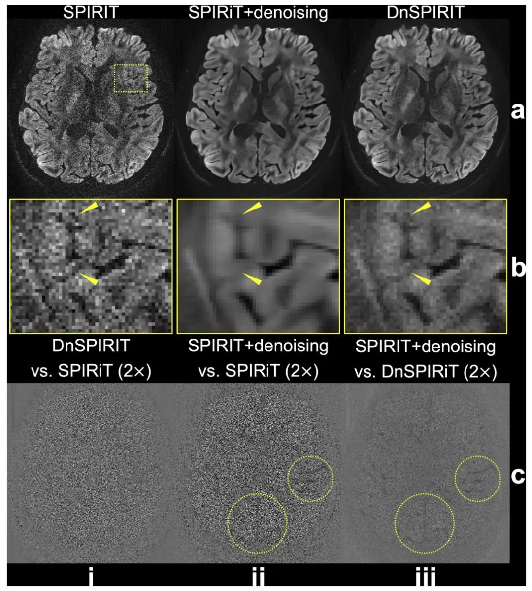
Fig. 2. Comparison of image reconstruction and processing strategies. In-vivo diffusion-weighted data (b = 1000 s/mm2 ) from 3T 0.65 mm protocol along (− 0.45, − 0.83, 0.32) are reconstructed using SPIRiT (a, i), SPIRiT followed by standalone BM4D denoising (SPIRiT+denoising, a, ii), and denoiser-regularized SPIRiT (DnSPIRiT, a, iii), with an enlarged region showing the image detail (b). Yellow arrows indicate regions where anatomical structures appear blurred in SPIRiT+denoising but are better preserved by DnSPIRiT. The difference maps between DnSPIRiT and SPIRiT (c, i), SPIRiT+denoising and SPIRiT (c, ii), SPIRiT+denoising and DnSPIRiT are also shown to illustrate the distribution of noise and structural differences (highlighted by yellow circles) across methods.
图2 图像重建与处理策略对比。基于3T 0.65毫米协议、扩散方向为(−0.45, −0.83, 0.32)的在体扩散加权数据(b=1000秒/平方毫米),分别采用以下三种方式重建:SPIRiT重建(a,i)、SPIRiT重建后进行独立BM4D去噪(SPIRiT+去噪,a,ii)、去噪器正则化SPIRiT重建(DnSPIRiT,a,iii);放大区域展示图像细节(b)。黄色箭头指示SPIRiT+去噪方法中解剖结构出现模糊、而DnSPIRiT方法能更好保留结构细节的区域。同时展示了以下差异图:DnSPIRiT与SPIRiT的差异图(c,i)、SPIRiT+去噪与SPIRiT的差异图(c,ii)、SPIRiT+去噪与DnSPIRiT的差异图,以阐明不同方法间噪声分布及结构差异(黄色圆圈突出显示)。

Fig. 3. Retrospective under-sampled reconstruction. Retrospective under-sampling is applied to the fully sampled data (i) from 3T 0.65 mm protocol by selecting 3 segments (Reff=2, ii) and 2 segments (Reff=3, iii) from the total of 6 segments. The diffusion-weighted images along direction (− 0.45, − 0.86, − 0.23) reconstructed using SPIRiT (a) and DnSPIRiT © and their difference with fully sampled reference (b, d) are shown to demonstrate the under-sampled reconstruction fidelity. The normalized root mean squared errors (NRMSE) between the under-sampled reconstructed image and the fully sampled reference of the whole slab are calculated within a brain mask to quantify their similarity
图3回顾性欠采样重建。对3T 0.65毫米协议的全采样数据(i)进行回顾性欠采样处理,从总共6个分段中选取3个分段(有效加速因子Rₑff=2,ii)和2个分段(有效加速因子Rₑff=3,iii)。展示了沿扩散方向(−0.45, −0.86, −0.23)的扩散加权图像,分别采用SPIRiT(a)和DnSPIRiT(c)重建的结果,以及重建图像与全采样参考图像的差异图(b、d),以验证欠采样重建的保真度。在脑掩模内计算欠采样重建图像与全采样参考图像的全块归一化均方根误差(NRMSE),用于量化二者的相似度。
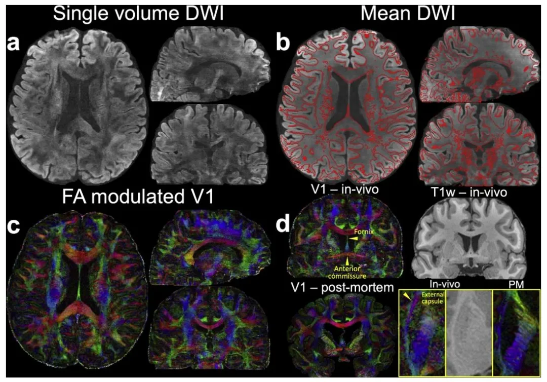
Fig. 4. Data from 3T 0.65 mm protocol. (a) In-vivo diffusion data (b = 1000 s/mm2 ) including diffusion-weighted image (DWI) along (− 0.45, 0.83, − 0.32), (b) 6- direction mean DWI with gray-white matter boundary derived from the T1w image using overlayed, © fractional anisotropy (FA) modulated V1 at 0.65 mm isotropic resolution, (d) a representative sagittal view of the FA modulated V1 (V1 – in-vivo) alongside the T1-weighted image (T1w – in-vivo), highlighting key structures including the fornix, external capsule, and anterior commissure are presented. For comparison, post-mortem (PM) data (V1 – post-mortem) from previous studies (Tendler et al., 2022) are shown. Enlarged views of the external capsule from an axial plane are provided for both in-vivo and post-mortem data (d)
图4 3T 0.65毫米协议采集数据。(a) 在体扩散数据(b=1000秒/平方毫米),包括沿扩散方向(−0.45, 0.83, −0.32)的扩散加权图像(DWI);(b) 6方向平均扩散加权图像,叠加了源自T1加权图像的灰白质边界;© 各向异性分数(FA)调制的V1图(各向同性分辨率0.65毫米);(d) 展示了FA调制V1图的代表性矢状位视图(V1——在体)及对应的T1加权图像(T1w——在体),重点标注了穹窿、外囊和前连合等关键结构。为进行对比,同时展示了以往研究中的尸检(PM)数据(V1——尸检)(Tendler等人,2022);并提供了在体与尸检数据中外囊区域的轴位放大视图(d)。

Fig. 5. Comparison of 3T 0.65 mm and 1.22 mm isotropic resolution DTI. Two axial slices showing the internal capsule (i) and pons (ii), and a sagittal slice showing the cingulum bundle (iii) of FA modulated V1 of 0.65 mm (a) and 1.22 mm (b) isotropic resolution in-vivo diffusion data acquired at 3T are demonstrated. White arrows highlight the improved delineation of the cingulum bundle in the 0.65 mm data
图5 3T磁场下0.65毫米与1.22毫米各向同性分辨率弥散张量成像(DTI)对比。展示了3T磁场下采集的在体扩散数据中,0.65毫米(a)和1.22毫米(b)各向同性分辨率的各向异性分数(FA)调制V1图的两个轴位切片(分别显示内囊(i)和脑桥(ii))及一个矢状位切片(显示扣带回束(iii))。白色箭头突出显示0.65毫米数据在扣带回束描绘方面的改善。

Fig. 6. Data from 3T 0.53 mm protocol. (a) In-vivo diffusion data of two subjects (b = 1000 s/mm2 ) including diffusion-weighted image (DWI) along (0.5, − 0.86, 0.02), (b) 20-direction mean DWI with gray-white matter boundary derived from the T1w image using FSL’s “fast” overlayed, © FA modulated V1 at 0.53 mm isotropic resolution.
图63T 0.53毫米协议采集数据。(a) 两名受试者的在体扩散数据(b=1000秒/平方毫米),包括沿扩散方向(0.5, −0.86, 0.02)的扩散加权图像(DWI);(b) 20方向平均扩散加权图像,叠加了通过FSL软件“fast”工具从T1加权图像中提取的灰白质边界;© 各向异性分数(FA)调制的V1图(各向同性分辨率0.53毫米)。
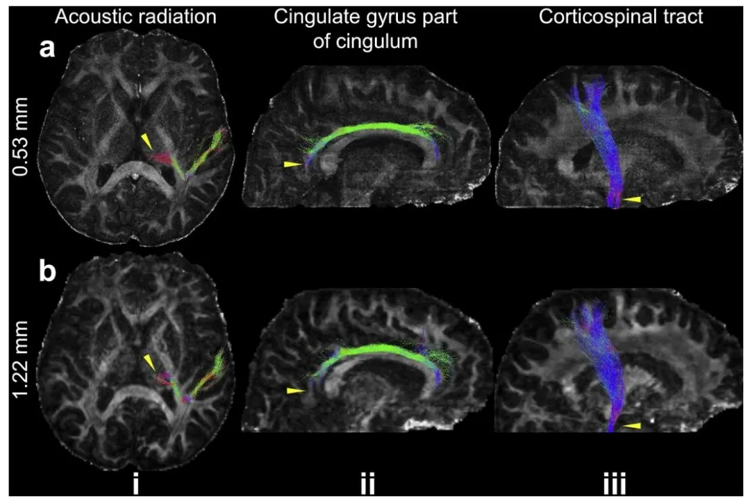
Fig. 7. Example white matter tracts from the 0.53 mm and 1.22 mm data. The maximum intensity projections of three representative white matter tracts including acoustic radiation (i), cingulate gyrus part of cingulum (ii), and corticospinal tract (iii) are overlayed on the fractional anisotropy maps of 0.53 mm (a) and 1.22 mm (b) datasets. The yellow arrows indicate the region where the tractography on 0.53 mm data shows improvement compared to that on 1.22 mm data.
图7 0.53毫米与1.22毫米数据的白质纤维束示例。将三组代表性白质纤维束(包括听辐射(i)、扣带回的扣带回部分(ii)和皮质脊髓束(iii))的最大强度投影图,叠加在0.53毫米(a)和1.22毫米(b)数据集的各向异性分数(FA)图上。黄色箭头指示0.53毫米数据的纤维束成像相较于1.22毫米数据有所改善的区域。

Fig. 8. Gyral bias comparison between 0.53 mm and 1.22 mm data. The fiber orientation distributions (FOD) (a, c) and tractography streamlines (b, d) for representative gyri from the 0.53 mm (i, iii) and 1.22 mm (ii, iv) data of two subjects are shown to demonstrate the reduced gyral bias on high-resolution data (highlighted by white arrows). Co-registered T1w images, along with enlarged T1w and fractional anisotropy (FA) maps (0.53 mm isotropic resolution) for the selected gyri, are provided as anatomical references to aid visualization of the cortical structure.
图8 0.53毫米与1.22毫米数据的脑回偏差对比。展示了两名受试者的0.53毫米(i、iii)和1.22毫米(ii、iv)数据中代表性脑回的纤维方向分布(FOD)(a、c)及纤维束成像流线(b、d),以体现高分辨率数据中脑回偏差的减少(白色箭头突出显示)。提供了配准后的T1加权图像,以及所选脑回的T1加权图像放大图和各向异性分数(FA)图(0.53毫米各向同性分辨率)作为解剖学参考,助力皮质结构的可视化。

Fig. 9. U-fibers comparison between 0.53 mm and 1.22 mm data. The whole-brain short association fibers tracked with one seed per voxel for 0.53 mm (a) and 1.22 mm (b) data are overlayed on fractional anisotropic maps. Representative enlarged regions (c-e) show the fiber orientation distributions (FOD) (i, iii), the tracked streamlines with one seed per voxel (ii, iv) for the 0.53 mm (i, ii) and 1.22 mm (iii, iv) data, and the tracked streamlines with 12 seeds per voxel for the 1.22 mm data (v) to compensate the difference in voxel numbers due to resolution. The white arrows indicate the region where the U-fibers on 0.53 mm data are better resolved at sharp turnings compared to that on 1.22 mm data.
图9 0.53毫米与1.22毫米数据的U型纤维对比。将0.53毫米(a)和1.22毫米(b)数据中全脑短联合纤维(每个体素设置一个种子点追踪)叠加在各向异性分数(FA)图上。代表性放大区域(c-e)展示了以下内容:0.53毫米(i、ii)和1.22毫米(iii、iv)数据的纤维方向分布(FOD)(i、iii)、每个体素一个种子点的追踪流线(ii、iv),以及1.22毫米数据中每个体素12个种子点的追踪流线(v)(用于补偿分辨率差异导致的体素数量不同)。白色箭头指示0.53毫米数据的U型纤维在急转区域相较于1.22毫米数据分辨率更高的区域。

Fig. 10. Comparisons of 7T 0.61 mm and 1.05 mm diffusion data. The sagittal, coronal, and axial slices of fractional anisotropy (FA) modulated V1 (a) and their enlarged regions (b, c) of 0.61 mm and 1.05 mm isotropic resolutions in-vivo diffusion data acquired at 7T are demonstrated, with white arrows highlighting the more detailed microstructure resolved by the high resolution at 0.61 mm. The traverse pontine fibers (d, i, ii) demonstrate similar patterns compared to previous postmortem study (d, iii, iv) (Tendler et al., 2022) at 0.5 mm isotropic resolution from the same scanner.
图10 7T磁场下0.61毫米与1.05毫米扩散数据对比。展示了7T磁场下采集的在体扩散数据中,0.61毫米和1.05毫米各向同性分辨率的各向异性分数(FA)调制V1图的矢状位、冠状位和轴位切片(a)及其放大区域(b、c),白色箭头突出显示0.61毫米高分辨率所解析的更精细微观结构。脑桥横纤维(d,i、ii)与以往在同一扫描仪上获取的0.5毫米各向同性分辨率尸检研究(d,iii、iv)(Tendler等人,2022)呈现出相似的形态特征。
Table
表
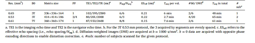
Table 1 Key parameters for submillimeter dMRI acquisition.
表1 亚毫米级扩散磁共振成像(dMRI)采集的关键参数
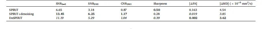
Table 2 Quantitative comparison of image reconstruction and processing strategies.** The performance of SPIRiT, SPIRiT followed by standalone BM4D denoising (SPIRiT+denoising), and denoiser-regularized SPIRiT (DnSPIRiT) is evaluated using six metrics: SNR of the b = 0 image (SNRb=0), SNR of diffusion-weighted images (SNRDWI, averaged across six DWIs), angular contrast-to-noise ratio (CNRDWI), image sharpness (normalized Tenengrad, averaged across six DWIs), and the absolute bias in white matter fractional anisotropy (FA) and whole-brain mean diffusivity (MD) relative to the 1.22 mm reference. The best and second-best values for each metric are highlighted in bold and italics, respectively.
表2 图像重建与处理策略的定量对比 评估了三种方法的性能:SPIRiT重建、SPIRiT重建后进行独立BM4D去噪(SPIRiT+去噪)、去噪器正则化SPIRiT重建(DnSPIRiT),采用六项指标:b=0图像的信噪比(SNRb=0)、扩散加权图像的信噪比(SNRDWI,取六幅扩散加权图像的平均值)、角度对比噪声比(CNRDWI)、图像锐度(归一化 tenengrad 梯度值,取六幅扩散加权图像的平均值)、白质各向异性分数(FA)的绝对偏差、全脑平均扩散系数(MD)相对于1.22毫米参考数据的绝对偏差。每项指标的最优值以粗体标注,次优值以斜体标注。