Title
题目
Compact programmable transmit scheme for contrast imaging using nonlinear difference-frequency ultrasound signals
基于非线性差频超声信号的紧凑型可编程造影成像发射方案
01
文献速递介绍
超声成像是一种经济高效且无创的技术,因其无电离辐射而被广泛应用于医疗领域,其用途涵盖众多应用场景(Andersen 等,2019)。然而,传统B型超声不适用于评估组织弹性,也难以穿透声阻抗失配较大的材料(Ihnatsenka 和 Boezaart,2010;Ozturk 等,2018;Schrenk 等,2020;Sigrist 等,2017)。 超声弹性成像解决了组织弹性评估的局限性,这一功能在癌症诊断和神经外科等应用中至关重要——在这些场景中,区分病变组织与健康组织的弹性或神经硬度具有关键意义(Sigrist 等,2017;Zardi 等,2020)。应变弹性成像是一种主流的超声弹性成像方法,需操作员手动对组织施加外部应力以测量产生的应变(Sigrist 等,2017;Zardi 等,2020;Carlsen 等,2013)。尽管该方法具备实时应用能力,但存在操作员依赖性强、主观性高及成像深度有限等缺点,这推动了替代弹性成像技术的发展(Ozturk 等,2018;Schrenk 等,2020;Sigrist 等,2017;Brunelli 等,2023)。 基于差频的超声弹性成像是其中一种替代技术。它利用两种基频超声信号的非线性相互作用生成第三种信号,其频率为两种基频的差值(Berntsen 等,1989;Ingard 和 Pridmore-Brown,1956;Li 等,2020;Westervelt,1957;Westervelt,1963;Thuras 等,1935)。这种相互作用在历史上被称为“声的声散射”(Ingard 和 Pridmore-Brown,1956;Westervelt,1957;Westervelt,1963)或“参量效应”(Westervelt,1963;Campo-Valera 等,2023),可用于估算介质的非线性系数,该系数与材料弹性相关。非线性系数表示为β=1+2B/A,而非线性参数B/A因材料不同而具有不同数值(Beyer,1960;Beyer,2008;Duck,2002;Mast,2000;Sehgal 等,1984)。已有研究对多种介质中这些参数的测量进行了探索,包括离体生物组织(Panfilova 等,2021;Nowicki 等,2024)。基于这种映射关系,可利用各种生物材料已知的非线性参数生成弹性成像造影图(Li 等,2020;Beyer,2008;Mast,2000;Sehgal 等,1984;Dunn 等,1981)。 基于差频的超声造影成像被称为振动声成像(VA)(de Oliveira 等,2021;Fatemi 和 Greenleaf,1998;Fatemi 和 Greenleaf,1999;Silva 和 Mitri,2011;Urban 等,2011)。在21世纪前二十年,VA在无损检测中的应用得到了广泛研究(de Oliveira 等,2021;Marcio 等,2021)。已有多项研究尝试通过各种信号处理方法改进VA(Marcio 等,2021;Urban 等,2015)。 Li 等(2020)提出了一种新型基于差频的超声造影成像技术,称为差频超声(dfUS),其相交角和差频均高于VA(Li 等,2020)。大相交角可使差频信号局域化,从而优化空间分辨率(Li 等,2020;Silva 和 Bandeira,2013)。与VA的千赫兹级差频不同,dfUS的差频处于兆赫兹级,这在牺牲穿透深度的前提下提高了对比度和分辨率。Li 等(2020)通过对多种离体目标的实验验证了dfUS的实际应用,包括小鼠胶质母细胞瘤的弹性成像造影。 VA和dfUS在超声弹性成像中均展现出良好前景,尤其适用于声阻抗失配显著的场景。传统线性超声受限于骨骼等材料的高声阻抗失配(Ihnatsenka 和 Boezaart,2010)。Agnollitto 等(2021)利用VA对健康小鼠、骨质疏松小鼠及经治疗的骨质疏松小鼠的离体股骨进行了检测和分类(Agnollitto 等,2021)。作者证实,VA具备利用超声成像骨骼及其内部结构的独特能力,而这一功能此前仅能通过磁共振、X射线成像等昂贵或有害的成像模态实现。更具体地说,dfUS允许在声阻抗存在显著差异的情况下进行超声弹性成像。 尽管VA和dfUS已成功应用于超声造影成像,但需降低这些技术的体积、复杂度和成本,才能将实验室成果转化为临床应用成效。现有关于dfUS和VA的研究通常采用三个独立换能器:两个基频换能器用于发射基频信号,第三个换能器用于检测这些频率的差值(Li 等,2020)。这导致电子转向难以实现,需进行机械扫描,且装置成本高、体积大。三个庞大且昂贵的换能器的焦点单独校准,进一步阻碍了dfUS从研究向临床的转化。 该问题的一种已知解决方案是整合这些换能器。例如,Fatemi 和 Greenleaf(1998)以及 Agnollitto 等(2021)采用带有两个单元的共焦换能器发射两种基频信号,并利用水听器检测差频信号(Fatemi 和 Greenleaf,1998;Agnollitto 等,2021)。尽管共焦换能器在一定程度上解决了体积和复杂度相关问题,但这些换能器的电子波束转向和聚焦能力有限或完全不具备。与 Li 等(2020)采用两个独立基频换能器的实验类似,使用共焦换能器时仍需机械转向和扫描方法,这进一步增加了成像深度、复杂度和扫描时间。为解决这些问题,需要一种能够实现电子转向和扫描的换能器阵列。 在此,我们提出一种新型dfUS发射方案,该方案采用可编程二维(2D)阵列探头,整合了两个基频换能器的发射功能。与以往方法不同,这种基于阵列的方法具有关键优势:可在紧凑且机械结构简单的装置中实现电子转向和扫描。由于用于发射基频信号的商用换能器带宽有限,本研究采用水听器检测差频信号。
Aastract
摘要
The nonlinear interaction between two acoustic waves at different primary frequencies generates a signal with a frequency equal to the difference between these primary frequencies. This signal is proportional to the nonlinear elasticity of the material being insonified; therefore, this signal can be used for elastographic contrast imaging. Previous studies on vibro-acoustography and difference-frequency ultrasound (dfUS) have used multiple separate low-element-count transducers for imaging, thereby increasing the bulk and complexity of the imaging system and necessitating mechanical steering and scanning. To address these limitations, we propose, demonstrate, and evaluate a novel array-based approach to difference-frequency-based ultrasound imaging. This 64-element ring array was constructed using a commercial 32 × 32 2D matrix array. This array-based scheme for dfUS imaging is customizable, programmable, and capable of electronic steering and scanning. The scheme generated traditional linear ultrasound and dfUS images of synthetic agarose and ex vivo phantoms. Statistical analysis of the results shows dfUS provides a 14.8 dB higher signal-to-noise ratio, 58.5% increased sensitivity, and 74.8 dB higher contrast compared to traditional linear ultrasound. In addition, a low mechanical index of 0.0248 was used in this preliminary study, thereby presenting opportunities for using transmit signals with increased strength in the future.
两种不同基频声波之间的非线性相互作用会产生一种频率等于这些基频差值的信号。该信号与被探测材料的非线性弹性成正比,因此可用于弹性成像造影。 此前关于振动声成像和差频超声(dfUS)的研究采用多个独立的少单元换能器进行成像,这增加了成像系统的体积和复杂度,且需要机械转向与扫描。为解决这些局限性,我们提出、验证并评估了一种新型基于阵列的差频超声成像方法。该64元环形阵列由商用32×32二维矩阵阵列构建而成,这种基于阵列的差频超声成像方案具有可定制、可编程特性,并能实现电子转向与扫描。 该方案对合成琼脂糖体模和离体体模进行了传统线性超声成像和差频超声成像。结果的统计分析表明,与传统线性超声相比,差频超声的信噪比提高14.8分贝,灵敏度提升58.5%,对比度提高74.8分贝。此外,本初步研究采用的机械指数仅为0.0248,为未来使用更高强度的发射信号提供了可能。
Method
方法
2.1. Theoretical background of dfUS
The bifrequency source of dfUS can be represented as
follows: p*(0, t) = p0asin(ωat) + p0bsin (ωbt), (1)
where p is the acoustic pressure of the source signal, p0a and p0b are the maximum acoustic pressures of the first and second primary-frequency signals, respectively, t is time, and ωa and ωb are the angular frequencies of the two primary-frequency signals (Blackstock et al., 2008). When the smaller of the two primary frequencies, ωb, is larger than the difference frequency, ω− = ωa − ωb*, the difference-frequency signal amplitude is as follows: p− (x, τ) = − βp0a**p0bω−2ρ0c30xsin(ω− ⋅τ), (2) where p− is the acoustic pressure of the difference frequency signal, x is the spatial variable, τ = t − x/c0 is the retarded time, where t is time and c*0 is the speed of small-signal sound, β = 1 + B/(2A) is the coefficient of nonlinearity, p0a and p0b are the source amplitudes of the two primary frequencies, and ρ0 is the ambient density (Blackstock et al., 2008).The above equation can be rewritten for calculating the coefficient of nonlinearity, β, as follows:
β = − 2ρ0c30xsin(ω− ⋅τ) ( p−p0ap0b*)(3)
Measurement at a set location ensures that x is constant, and using the maximum pressure over time removes the sine function from the denominator. As both ρ0 and c0 of water are known, the only values that must be measured empirically are p− of the difference-frequency signal and p0a and p0b of the primary-frequency signals. Therefore, if we measure these three values and normalize p− using p0ap0b, we can estimate the coefficient of nonlinearity corresponding to a given location. This process was repeated by mechanical scanning from different places, and displaying p− /(p0ap0b*) generated an elastographic contrast image with the normalization equation being expressed as the following: γΔf,normalized = ∑1.5Δf0.5Δf|P(f)||P(f1)|⋅|P(f*2)|, (4) where P(f) is the FFT of the pressure at frequency f, P(f1) is the FFT of the pressure at frequency f1, P(f2) is the FFT of the pressure at frequency f**2, and Δf is the difference frequency f1 − f2. By extracting frequencydomain data from Eq. (4), obtaining a quantitative estimate of the coefficient of nonlinearity at each target point is possible, allowing the ability to create an elastographic contrast image.
2.1 差频超声(dfUS)的理论基础 差频超声的双频声源可表示为: [ p*(0, t) = p{0a}\sin(\omega_a t) + p{0b}\sin(\omega_b t) \tag{1} ] 其中,( p ) 表示声源信号的声压,( p{0a} ) 和 ( p{0b} ) 分别为两种基频信号的最大声压,( t ) 为时间,( \omega_a ) 和 ( \omega_b ) 为两种基频信号的角频率(Blackstock 等,2008)。当两种基频中较小的角频率 ( \omega_b ) 大于差频 ( \omega- = \omega_a - \omega_b ) 时,差频信号的振幅可表示为: [ p-(x, \tau) = -\beta p{0a} p{0b} \omega-2 \rho_0 c_03 x \sin(\omega- \cdot \tau) \tag{2} ] 其中,( p- ) 为差频信号的声压,( x ) 为空间变量,( \tau = t - x/c_0 ) 为延迟时间(( t ) 为时间,( c_0 ) 为小信号声速),( \beta = 1 + B/(2A) ) 为非线性系数,( \rho_0 ) 为环境密度(Blackstock 等,2008)。 通过改写上述方程,可得到非线性系数 ( \beta ) 的计算公式: [ \beta = -\frac{2\rho_0 c_03}{x \sin(\omega- \cdot \tau) \cdot (p- p{0a} p{0b})} \tag{3} ] 在固定位置测量时,( x ) 为常量;取随时间变化的最大声压可消去分母中的正弦函数。由于水的 ( \rho_0 ) 和 ( c_0 ) 为已知量,仅需通过实验测量差频信号的 ( p- ) 以及两种基频信号的 ( p{0a} ) 和 ( p{0b} )。因此,测量这三个参数并利用 ( p{0a} p{0b} ) 对 ( p- ) 进行归一化后,即可估算对应位置的非线性系数。 通过在不同位置进行机械扫描重复上述过程,并显示 ( p-/(p{0a} p{0b}) ),可生成弹性成像造影图,其归一化方程如下: [ \gamma{\Delta f, \text{normalized}} = \sum{0.5\Delta f}^{1.5\Delta f} \frac{|P(f)|}{|P(f_1)| \cdot |P(f_2)|} \tag{4} ] 其中,( P(f) ) 为频率 ( f ) 处声压的快速傅里叶变换(FFT)结果,( P(f_1) ) 和 ( P(f_2) ) 分别为基频 ( f_1 ) 和 ( f_2 ) 处声压的FFT结果,( \Delta f = f_1 - f_2 ) 为差频。通过提取式(4)的频域数据,可定量估算每个目标点的非线性系数,进而生成弹性成像造影图。 要不要我帮你整理一份dfUS核心公式说明表,清晰列出各公式的用途、关键参数定义及应用场景?
Conclusion
结论
An array-based dfUS scheme was successfully designed and implemented in this study. This system is highly programmable, customizable, compact, safe for clinical use, and capable of electronic steering and scanning. The obtained images confirmed that the signal-to-noise ratio, sensitivity, and contrast were higher than those obtained using conventional linear ultrasound. The resultant images apparently show that dfUS has a 14.8 dB higher signal-to-noise ratio, 58.5 % improved sensitivity, and 74.8 dB greater contrast compared to conventional linear ultrasound. The improvement in these factors demonstrates the potential of using dfUS in ultrasound elastography, mainly when highacoustic-impedance mismatches are involved. Future work will integrate the receiving and transmitting transducer into the scheme for detecting the differences in frequency, thereby increasing the compactness and reducing the cost of the setup. This integration aims toenhance system compactness and reduce costs by eliminating the need for a separate hydrophone to detect frequency differences, allowing the transducers to operate in reflection mode. Future iterations may also explore the use of an annular array comprising concentric rings, each dedicated to one of the primary frequencies. This configuration will consolidate the functionalities of the two primary-frequency transducers and the receiver, as demonstrated in this study, thereby negating the need for an external hydrophone. Another area of improvement, given the low 38 % fractional bandwidth’s effects on resolution and signal strength, is to use a wide-bandwidth transducer such as a capacitive micromachined ultrasonic transducer, which has increased performance compared to conventional bulk piezoelectric transducers (Huh et al., 2024). Furthermore, the mechanical index of 0.0248 observed in our experiments is well within safe limits, suggesting the feasibility of employing a more powerful transducer to enhance imaging quality. Increasing the strength of the transmitted primary frequency signals could effectively compensate for the inherently low magnitude of dfUS signals, potentially unlocking new possibilities in high-resolution ultrasound imaging.
本研究成功设计并实现了一种基于阵列的差频超声(dfUS)方案。该系统具有高度可编程性、可定制性,结构紧凑且适用于临床安全场景,同时具备电子转向和扫描功能。成像结果证实,其信噪比、灵敏度和对比度均优于传统线性超声——与传统线性超声相比,dfUS的信噪比提高14.8分贝,灵敏度提升58.5%,对比度增加74.8分贝。这些性能指标的提升,彰显了dfUS在超声弹性成像中的应用潜力,尤其适用于声阻抗失配显著的场景。 未来研究将把接收换能器与发射换能器整合到差频检测方案中,通过省去单独的水听器、使换能器工作在反射模式,进一步提升系统紧凑性并降低成本。后续迭代版本还可能探索采用环形阵列(由同心环组成,每个环专门对应一种基频),这种结构将整合本研究中两种基频换能器与接收器的功能,从而无需外部水听器。此外,鉴于38%的低相对带宽对分辨率和信号强度的影响,另一改进方向是采用宽带换能器(如电容式微机械超声换能器),其性能优于传统体压电换能器(Huh等,2024)。 值得注意的是,本实验中测得的机械指数为0.0248,远在安全范围内,这表明采用功率更强的换能器以提升成像质量具有可行性。增强基频发射信号的强度,可有效补偿dfUS信号固有的低幅度特性,有望为高分辨率超声成像开辟新的可能。 要不要我帮你整理一份dfUS方案核心优势与未来优化方向清单,清晰梳理其技术亮点及后续改进重点?
Results
结果
3.1. Verifying the transmit scheme
First, the dfUS scheme’s ability to transmit and focus ultrasounds was verified. Fig. 3 shows various focal points obtained in deionized and degassed water. All 52 transducer elements transmitted a 7.81 MHz ultrasonic pulse along the Z-axis, with the XY-plane parallel to the transducer. As shown in Fig. 3(a), the natural focus is 23 mm from the transducer.The scheme’s ability to electronically change the focus was verified by imaging two additional focal points at 25 and 33 mm, as shown in Fig. 3(b) and ©, respectively. Fig. 3(d) and (e) show the ultrasound signals in Fig. 3(b) traveling along the XZ- and YZ-planes, respectively. In addition, all three focal points were well-defined, proving the programmability and electronic steering capability of the dfUS transmit scheme.The peak positive and negative pressures were measured to be 79.2 and 69.3 kPa, respectively. The latter corresponded to a mechanical index of 0.0248, which is well below the Food and Drug Administrationmandated maximum mechanical index of 1.9; therefore, our dfUS scheme can generally be considered safe for testing human subjects (Deng et al., 2015; Patton et al., 1994). In addition, this scheme can be expanded and improved via tests to achieve increased mechanical indices, which can improve image quality.In the case of a single-period transmission, the actual transmitted frequency differs from the frequency set in the software. Fig. 3(f) and (g) show the filtered hydrophone signals in the time and frequency domains, respectively, with the latter showing the detected peak frequency. Supplementary Fig. 1(a) and (b) show this discrepancy in frequencies, which is resolved for the difference-frequency transmission shown in Fig. 4(e). We suspect that a long transmit pulse might remove the discrepancy between the excitation signal and the recorded hydrophone signal with the low bandwidth of the transducer. A single-period sine wave at 7.8125 MHz was used to excite the transducer, with the hydrophone signal shown in Supplementary Fig. 1©. Despite the excitation frequency being close to the center frequency of the transducer, the frequency-domain analysis shown in Supplementary Fig. 1(d) shows that the actual center frequency of the recorded waveform is centered at 6.18 MHz. The − 3 dB points are located at 5 and 7.36 MHz, giving a − 3 dB fractional bandwidth of 38 %. To compensate for this issue, we used longer excitation signals of up to 20 long periods to force the transducer to the desired frequencies and increase the magnitude of the difference-frequency signals. This would come at the cost of axialresolution, but as we are not scanning in the axial direction in this study, we deemed it an acceptable interim solution while we source a widebandwidth transducer.Based on the proven electronic focusing capability of the dfUS scheme, it must be determined whether a difference in frequencies is generated and focused properly. The measured differences in the frequency signals are shown in Fig. 4. Fig. 4(a)–© show the sum of the spectral powers of the different frequencies in the XY-plane at their respective focuses of 23 mm (the natural focus), 25 mm, and 33 mm. To account for the transmitted signal bandwidth and errors in the transmitted frequencies, the difference frequency was assigned a 50 % tolerance in either direction. This translates to a frequency range of 0.78–2.35 MHz, and the spectral powers of these frequencies were summed to obtain the images in Fig. 4(a)–©.Although the dfUS scheme should allow for good electronic steering and scanning across a wide range of depths, dfUS imaging may have an optimal depth. Fig. 4(d) shows the full widths at half maximum (FWHMs) of the difference frequency signals at various focal points. The − 3 dB points, which corresponded to the FWHMs when the transducer was used in the reflection mode, were 1.06, 0.954, and 1.85 mm obtained from the 23, 25, and 33 mm tests, respectively. A small FWHM indicates a highly focused beam from the dfUS signal, enabling imaging with high lateral resolution. The dynamic ranges were 12.7, 29.0, and 7.96 dB for the 23, 25, and 33 mm tests, respectively. A large dynamic range indicates that the amplitude of the central dfUS beam is larger than those of the side lobes and the background noise levels. As the dfUS image at 25 mm had both the largest dynamic range and the smallest FWHM, the focal point at Z = 25 mm was used for subsequent dfUS experiments. Fig. 4(e) and (f) show the time- and frequency-domain aspects of the signal, respectively. The long 20-period pulses, shown in Fig. 4(e), were used in the difference-frequency experiments because the transmitted primary frequencies must match the intended frequencies. Owing to hardware limitations, the actual transmitted frequency differed from the frequency set in the software. As shown in Supplementary Fig. 1, this issue was resolved by transmitting long pulses.
3.1 发射方案验证 首先,对差频超声(dfUS)方案的超声发射与聚焦能力进行了验证。图3展示了在去离子脱气水中获得的多个焦点。全部52个换能器单元沿Z轴发射7.81 MHz超声脉冲,XY平面与换能器平行。如图3(a)所示,其自然焦点位于距换能器23 mm处。 通过对25 mm和33 mm处的另外两个焦点进行成像,验证了该方案电子调焦能力,结果分别如图3(b)和©所示。图3(d)和(e)分别展示了图3(b)中超声信号沿XZ平面和YZ平面的传播情况。此外,三个焦点均轮廓清晰,证实了dfUS发射方案的可编程性和电子转向能力。 测量得到的正负峰值压力分别为79.2 kPa和69.3 kPa,后者对应的机械指数为0.0248,远低于美国食品药品监督管理局(FDA)规定的最大机械指数1.9,因此该dfUS方案基本可认为适用于人体受试测试(Deng等,2015;Patton等,1994)。此外,通过进一步测试可扩展和改进该方案以提高机械指数,从而改善成像质量。 在单周期发射情况下,实际发射频率与软件设定频率存在差异。图3(f)和(g)分别展示了水听器信号在时域和频域的滤波结果,后者显示了检测到的峰值频率。补充图1(a)和(b)展示了这种频率差异,而图4(e)所示的差频发射中该差异得到解决。我们推测,由于换能器带宽较低,较长的发射脉冲可能消除激励信号与记录的水听器信号之间的差异。使用7.8125 MHz的单周期正弦波激励换能器,水听器信号如补充图1©所示。尽管激励频率接近换能器的中心频率,但补充图1(d)的频域分析显示,记录波形的实际中心频率为6.18 MHz,其-3 dB点位于5 MHz和7.36 MHz处,对应的-3 dB相对带宽为38%。为解决这一问题,我们使用了长达20个周期的激励信号,以迫使换能器工作在目标频率并提高差频信号的幅度。这会牺牲轴向分辨率,但由于本研究未在轴向方向进行扫描,我们认为这是一种可接受的临时解决方案,同时正在寻找宽带换能器。 基于已证实的dfUS方案电子聚焦能力,还需确定是否能生成差频并实现有效聚焦。图4展示了测量得到的差频信号。图4(a)-©分别显示了在23 mm(自然焦点)、25 mm和33 mm焦点处,XY平面内不同频率的频谱功率总和。考虑到发射信号带宽和发射频率误差,差频允许有±50%的容差,对应频率范围为0.78-2.35 MHz,对这些频率的频谱功率求和得到图4(a)-©中的图像。 尽管dfUS方案应能在较宽深度范围内实现良好的电子转向和扫描,但dfUS成像可能存在最佳深度。图4(d)展示了不同焦点处差频信号的半高全宽(FWHM)。换能器工作在反射模式时,23 mm、25 mm和33 mm测试点对应的-3 dB点(即FWHM)分别为1.06 mm、0.954 mm和1.85 mm。较小的FWHM表明dfUS信号波束聚焦性强,可实现高横向分辨率成像。23 mm、25 mm和33 mm测试点的动态范围分别为12.7 dB、29.0 dB和7.96 dB。较大的动态范围表明中心dfUS波束的幅度远大于旁瓣和背景噪声。由于25 mm处的dfUS图像同时具有最大动态范围和最小FWHM,后续dfUS实验均采用Z=25 mm处的焦点。图4(e)和(f)分别展示了信号的时域和频域特性。图4(e)所示的20周期长脉冲用于差频实验,以确保发射的基频与目标频率一致。由于硬件限制,实际发射频率与软件设定频率存在差异,如补充图1所示,这一问题通过发射长脉冲得到解决。
Figure
图

Fig. 1. Difference-frequency ultrasound (dfUS) scheme and artist’s impressions of the resultant ultrasound images. Overall scheme of dfUS imaging is shown on the left. Bone structure, including the bone marrow, is shown in the middle, and the two right images show the resulting linear ultrasound (top) and dfUS image (bottom).
图1 差频超声(dfUS)成像方案及超声成像结果示意图。左侧为dfUS成像整体方案,中间为包含骨髓的骨骼结构示意图,右侧两张图分别为传统线性超声成像结果(上图)和dfUS成像结果(下图)。
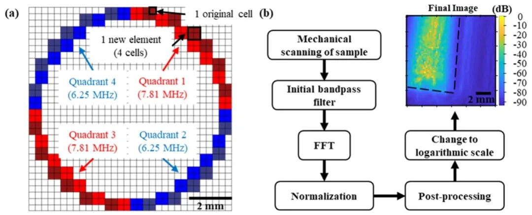
Fig. 2. Overview of the dfUS transmit and imaging schemes. a, dfUS transmit scheme. Original 300 μm × 300 μm cells and new selected ring-type array elements are shown. Starting from the topmost red element and going clockwise, the elements are numbered from 1 to 52. The elements in quadrants 1 and 3, shown in red, transmit f1 = 7.81 MHz, while the elements in quadrants 2 and 4, shown in blue, transmit f2 = 6.25 MHz. b, Flowchart of dfUS raw data acquisition, processing, and imaging
图2 差频超声(dfUS)发射及成像方案总览。a为dfUS发射方案,展示了原始300微米×300微米的单元及新选定的环形阵列单元;从最上方红色单元开始顺时针编号,1-52号为阵列单元,红色标注的1、3象限单元发射频率f₁=7.81兆赫兹,蓝色标注的2、4象限单元发射频率f₂=6.25兆赫兹。b为dfUS原始数据采集、处理及成像的流程图。
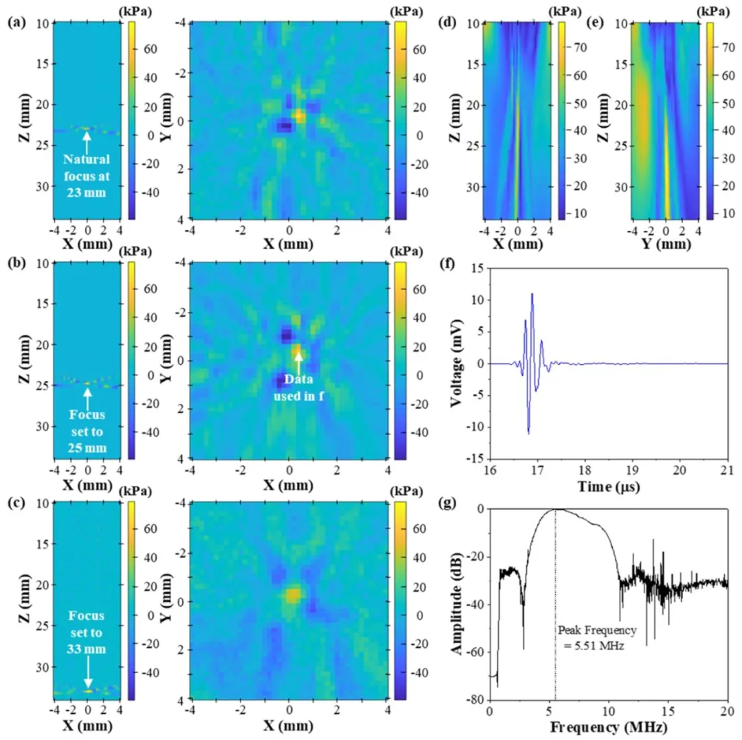
Fig. 3. Hydrophone data from various adjustable focal points obtained in a tank containing deionized and degassed water with a single-frequency transmission at 7.81 MHz. Z represents the distance from the transducer. a, Frame of data showing the natural focus at 23 mm in the XZ-plane (left) and XY-plane (right). b, Frame of data showing the focus at 25 mm in the XZ-plane (left) and XY-plane (right). c, Frame of data showing the focus at 33 mm in the XZ-plane (left) and XY-plane (right). d, Maximum pressure in the XZ-plane, showing the direction of travel of the ultrasound beam from the transducer with the focus set at Z = 25 mm. e, Maximum pressure in the YZ-plane, showing the direction of travel of the ultrasound beam from the transducer with the focus set at Z = 25 mm. f, Time-domain representation of the focal point used in this study obtained from the data point marked in (b). g, Fast Fourier transform of the data shown in (f). Note that the transmitted frequency is not at the expected frequency because only one period is transmitted. Supplementary Figure 1 shows the difference between the transmitted and actual frequencies.
图3 在装有去离子脱气水的水槽中,以7.81兆赫兹单频发射时,不同可调焦点的水听器数据。Z表示距换能器的距离。a为XZ平面(左)和XY平面(右)内23 mm处自然焦点的数据帧;b为XZ平面(左)和XY平面(右)内25 mm处焦点的数据帧;c为XZ平面(左)和XY平面(右)内33 mm处焦点的数据帧;d为XZ平面内的最大压力分布,展示焦点设定为Z=25 mm时超声束从换能器的传播方向;e为YZ平面内的最大压力分布,展示焦点设定为Z=25 mm时超声束从换能器的传播方向;f为从(b)中标记的数据点获取的本研究所用焦点的时域波形;g为(f)中数据的快速傅里叶变换(FFT)结果。注:由于仅发射一个周期,实际发射频率与预期频率存在差异,补充图1展示了发射频率与实际频率的差值。

Fig. 4. Hydrophone data from various adjustable focal points obtained in a tank containing deionized and degassed water with a dual transmission frequency of 7.81 MHz and 6.25 MHz. Z represents the distance from the transducer. a, XY-plane image showing the spectral power of the dfUS signal in the XY-plane obtained at Z =23 mm with a focus set to the natural focus at 23 mm. b, XY-plane image showing the spectral power of the dfUS signal in the XY-plane obtained at Z = 25 mm with a focus set at 25 mm. c, XY-plane image showing the spectral power of the dfUS signal in the XY-plane obtained at Z = 33 mm with a focus set at 33 mm. d, Analysis of the − 3 dB points obtained from the point spread functions of (a)–©. The distances between the − 3 dB points are 1.06, 0.954, and 1.85 mm obtained from the 23, 25, and 33 mm tests, respectively. e, Time-domain representation of the received hydrophone signal obtained from the focus at X = 0 mm, Y = 0 mm, Z = 25 mm, as shown in (b). f, Fast Fourier transform of the signal shown in (f).
图4 在装有去离子脱气水的水槽中,以7.81兆赫兹和6.25兆赫兹双频发射时,不同可调焦点的水听器数据。Z表示距换能器的距离。a为焦点设定于23 mm(自然焦点)时,在Z=23 mm处获取的dfUS信号在XY平面的频谱功率图像;b为焦点设定于25 mm时,在Z=25 mm处获取的dfUS信号在XY平面的频谱功率图像;c为焦点设定于33 mm时,在Z=33 mm处获取的dfUS信号在XY平面的频谱功率图像;d为(a)-©中点扩散函数的-3 dB点分析结果,23 mm、25 mm和33 mm测试对应的-3 dB点间距分别为1.06 mm、0.954 mm和1.85 mm;e为(b)中X=0 mm、Y=0 mm、Z=25 mm焦点处接收的水听器信号时域波形;f为(e)中信号的快速傅里叶变换(FFT)结果。
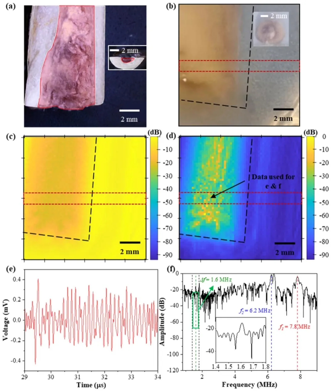
Fig. 5. a, Chicken-bone sample in (b)–(d) cut parallel to the image plane. The bone marrow is highlighted in red, and the bone is highlighted in white. b, Image of the chicken-bone phantom, showing both the bone and bone marrow. The black dashed lines in (b)–(d) outline the phantom, whereas the areas outlined in red are used to calculate SNR. Inset image shows a side view. c, Normalized acoustic pressure obtained from a single-frequency transmission at 7.81 MHz. Both © and (d) are scaled for a 94 dB range. d, dfUS signal normalized similar to ©. For both © and (d), the bottom of the chicken-bone phantom and the hydrophone are placed 24 and 50 mm from the hydrophone, respectively. e, Time-domain representation of the dfUS hydrophone data corresponding to the marked pixel in (d). f, Frequencydomain representation of the data in (e). The inset graph shows a magnified view around the difference frequency
图5 a为(b)-(d)中与成像平面平行切割的鸡骨样本,红色高亮显示骨髓,白色高亮显示骨骼;b为鸡骨体模图像,同时呈现骨骼和骨髓结构,(b)-(d)中黑色虚线勾勒体模轮廓,红色勾勒区域用于计算信噪比(SNR),插图为侧视图;c为7.81兆赫兹单频发射时获得的归一化声压图像,©和(d)均按94分贝范围缩放;d为与©采用相同归一化方式的dfUS信号图像,鸡骨体模底部和水听器距换能器的距离分别为24 mm和50 mm;e为(d)中标记像素对应的dfUS水听器数据时域波形;f为(e)中数据的频域表征,插图为差频附近的放大视图。
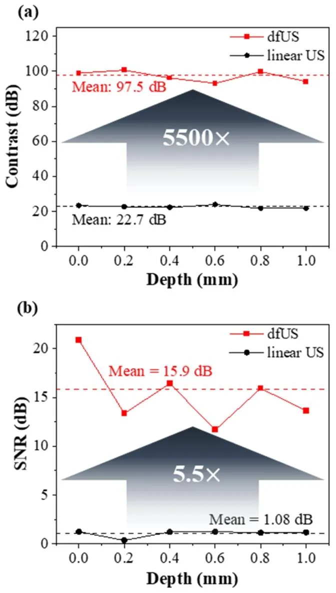
Fig. 6. Maximum contrast and SNR analysis. a, Comparison of the contrasts obtained using linear ultrasound and dfUS at various depths. b, Comparison of the signal-to-noise ratios (SNR) obtained using linear ultrasound and dfUS at various depths. The SNR is calculated from the areas within the red dashed lines in Fig. 5b–d.
图6 最大对比度与信噪比(SNR)分析。a为不同深度下传统线性超声与dfUS的对比度对比;b为不同深度下传统线性超声与dfUS的信噪比对比,其中信噪比基于图5b-d中红色虚线框内区域计算得出。
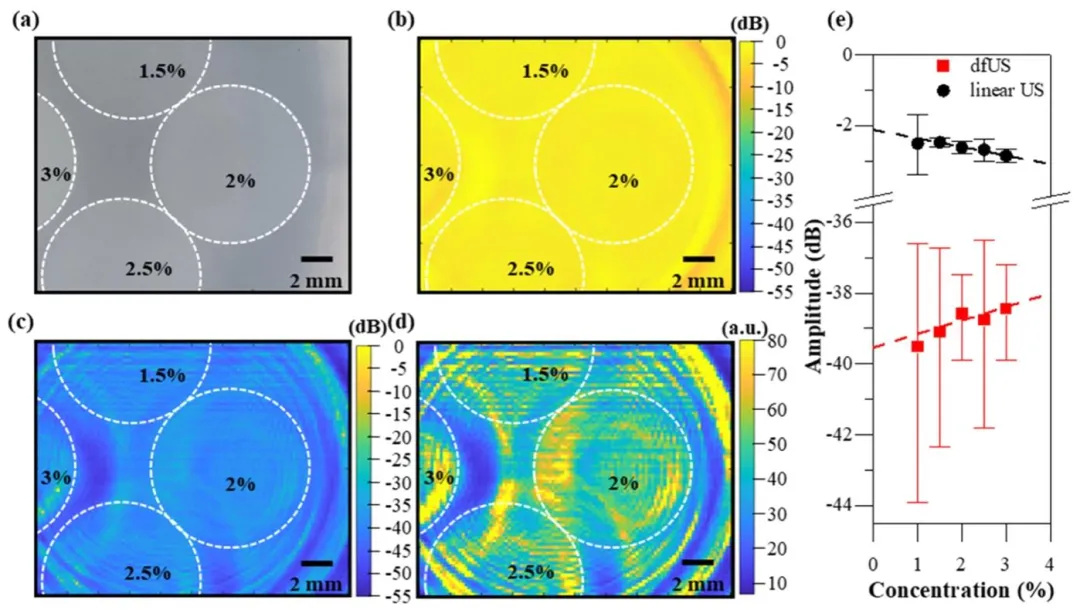
Fig. 7. Demonstration of the ability of dfUS to differentiate between materials with small elasticity contrasts. a, Image showing four 8-mm-diameter agarose targets. Clockwise from the top: 1.5, 2, 2.5, and 3 wt. % agarose. b, Linear ultrasound image of (a) with logarithmic compression. c, dfUS image of (a) with logarithmic compression. d, dfUS image of (a) with power-law compression. e, Mean and standard deviations of all points within 3 mm of the center points of each target in black (b) and red © normalized to the maximum value for each image. Error bars denote standard deviation, and the dotted lines show linear fits.
图 7 差频超声(dfUS)区分低弹性对比度材料的能力验证。a 为四个直径 8 毫米的琼脂糖目标样本图像,从顶部顺时针依次为 1.5%、2%、2.5% 和 3% 重量百分比的琼脂糖;b 为 (a) 的传统线性超声图像(采用对数压缩);c 为 (a) 的 dfUS 图像(采用对数压缩);d 为 (a) 的 dfUS 图像(采用幂律压缩);e 为 (b) 中黑色标记区域和 © 中红色标记区域内,各目标中心点 3 毫米范围内所有像素点的均值与标准差(均相对于各图像最大值归一化),误差棒表示标准差,虚线为线性拟合曲线。