Title
题目
Recovering intrinsic conduction velocity and action potential duration fromelectroanatomic mapping data using curvature
基于曲率从电解剖标测数据中恢复固有传导速度与动作电位时程
01
文献速递介绍
电解剖标测系统相关研究内容翻译 电解剖标测系统能在更短时间内实现更高密度的心脏激动标测。这类标测图可识别出缓慢传导区域,这些区域可能是潜在的治疗靶点。但心肌纤维结构会使标测图的解读变得复杂(Vigmond等,2025),进而形成复杂的激动模式。通过分析动作电位时程(APD)的替代指标——激动恢复间期(ARI),还可从电解剖标测图中提取APD,从而识别致心律失常风险区域(Orini等,2020)。 长期以来,曲率一直被视为影响心脏传导的重要因素。在分析电活动标测图时,波前曲率是需重点考量的方面,因为它会同时影响传导速度(CV)(Wellner等,2002;Fast和Kléber,1997)与APD(Comtois和Vinet,1999;Qu等,2000)。高曲率值可能导致局部传导阻滞,为折返心律的形成创造条件(Cabo等,1998)。同样,波后曲率会调节APD,使复极梯度变陡——这一过程具有致心律失常性,且可能诱发室性早搏(Zhang等,2024)。 人们通常仅从激动波前的形状角度理解曲率,但在心脏组织中,纤维结构会改变局部物质坐标系,导致波前的有效法线与几何法线不再重合(Dierckx等,2011)。曲率为正值时,表明波前局部呈凸面,此时电流 sinks 大于源电流;曲率为负值时,则情况相反。凸面波前会使CV减慢,APD也随之延长。凸面波前导致传导速度降低的原因是:离开波前的电流面临更大的表面积,电流密度随之降低,因此需要更长时间才能使下游细胞膜充电至兴奋阈值。 传导速度与曲率的关系可用线性方程描述(Fast和Kléber,1997),而APD与曲率的关系则更为复杂(Comtois和Vinet,1999)。心脏组织的各向异性结构同样会影响曲率计算:与CV在纤维方向上传导更快类似,各向异性曲率在纤维方向上的数值也小于其垂直方向(Colli Franzone等,2014)。 曲率是在药物作用、电重构或基质改良基础上产生的动态调节效应,其大小由起搏位置及后续激动模式决定。当试图通过计算模型评估致心律失常潜力时,参数赋值需要依赖组织的固有特性——即离体细胞所表现出的特性。但遗憾的是,在生物学测量中,这些固有特性会被上述因素掩盖。 因此,在分析临床激动时间标测图时,考虑曲率影响至关重要:由凸面波前导致的缓慢传导,可能会与钠电流受损或缝隙连接表达降低的区域相混淆。在分析激动恢复间期(ARI)标测图时(Yang等,2018),复极离散度的部分成因可能源于曲率,从而掩盖了组织的固有差异。 了解曲率对CV和APD的影响后,我们可将这一认知整合到传导与复极模型中,更精准地复现组织中的激动模式,并恢复细胞的固有特性。本文中,我们在几何真实的心脏组织模型中,研究了曲率对传导速度和APD的影响;通过二维和三维模型示例,展示了如何从记录的临床标测图中确定固有APD与固有CV。
Aastract
摘要
Electroanatomic mapping systems measure the spread of activation and recovery over the surface of the heart.Propagation in cardiac tissue is complicated by the tissue architecture which produces a spatially varyinganisotropic conductivity, leading to complex wavefronts. Curvature of the wavefront is known to affect bothconduction velocity (CV) and action potential duration (APD). In this study, we sought to better define theimpact of wavefront curvature on these properties, as well as the influence of conductivity, in order to recoverintrinsic tissue properties. The dependence of CV and APD on curvature were measured for positive andnegative curvatures for several ionic models, and then verified in realistic 2D and 3D simulations. Clinical datawere also analysed. Results indicate that the effects of APD and CV are well described by simple formulae,and if the structure of the fibre is known, the intrinsic propagation velocities can be recovered. Geometricalcurvature, as determined strictly by wavefront shape and ignoring the fibre structure, leads to large regionsof spurious high curvature. This is important for determining pathological zones of slow conduction. In thesimulations studied, curvature modulated APD by at most 20 ms.
电解剖标测系统相关研究内容翻译 电解剖标测系统可测量心脏表面激动与恢复过程的传导扩散情况。心脏组织中的电传导过程因组织结构而变得复杂——这种结构会导致电导率呈现空间异质性(各向异性),进而形成复杂的波前。已知波前曲率会同时影响传导速度(CV)与动作电位时程(APD)。 本研究旨在更清晰地明确波前曲率对上述特性的影响,以及电导率的作用,从而恢复组织的固有特性。研究针对多种离子模型,分别测量了正、负曲率下CV与APD对曲率的依赖关系,并在真实的二维(2D)和三维(3D)模拟中进行了验证,同时还分析了临床数据。 结果表明,APD与CV的变化可通过简单公式较好地描述;且若已知心肌纤维结构,即可恢复组织的固有传导速度。仅由波前形状决定、忽略纤维结构的几何曲率,会导致出现大范围的虚假高曲率区域。这一点对于识别缓慢传导的病理区域具有重要意义。在本研究的模拟实验中,曲率对APD的调制幅度最高不超过20毫秒。
Method
方法
2.1. Calculation of curvature
The curvature of a line is the inverse of the radius of the circletangent to the line. For a surface, there are two directions of curvature,along which a maximum and a minimum line curvature are computed,and we are interested in the sum of these two curvatures, 𝜅, referred toas twice the mean curvature (Keener and Sneyd, 2009). We start witha map of activation times, 𝜏(𝑥). For isotropic tissue, this curvature canbe computed as𝜅 = ∇ ⋅ ̂𝑛, (1)where ̂𝑛 is the outward normal of wavefront propagation as obtainedby normalizing the gradient of activation time, ‖ ∇𝜏∇𝜏‖ . For instance, aspherical front of radius 𝑟 has curvature 𝜅 = ±2𝑟, positive for expanding(convex) fronts and negative for contracting (concave) fronts.For cardiac tissue which is anisotropic, the monodomain conductivity tensor 𝐆 which depends on local fibre orientation modifies theexpression (Colli Franzone et al., 2005):𝜅 = ∇ ⋅ ( 𝐆̂𝑛√ ̂𝑛𝑇* 𝐆̂𝑛 ) . (2)and we shall refer to this as the anisotropic curvature. Given conductivities 𝜎𝐿 along the fibre direction ̂𝑓*, 𝜎𝑡 along the transverse direction𝑡̂, and 𝜎𝑠 in the sheet normal direction ̂𝑠:𝐆 = 𝜎𝐿̂𝑓 ⊗ ̂𝑓+ 𝜎𝑡 𝑡 ⊗̂ 𝑡̂+ 𝜎𝑠 ̂𝑠 ⊗ ̂𝑠, (3)where ⊗ denotes the outer product. The resultant propagation velocityis given by (Colli Franzone et al., 2005):𝜃 = 𝜃0 ⋅ (1 − 𝑐𝜅) (4)= 𝜃0 − 𝐷𝜅 (5)where 𝑐 is a constant, 𝜃0 is the speed of a planar wavefront, and 𝐷 isthe diffusion coefficient. (Note that in Colli Franzone et al. (2005) theformula for the curvature in Eq. (2) is with a minus and Eq. (4) is witha plus. Here, we assume the geometrical definition of curvature.) Thediffusion coefficient can also be evaluated from model parameters by𝐷* = 𝜎(𝑥)∕(𝛽𝐶𝑚) (6)where 𝛽 is the membrane surface-to-volume ratio, 𝐶𝑚 is the membranecapacitance (Colli Franzone et al., 2005), and 𝜎(𝑥) is the conductivityseen by the advancing wavefront. It follows that the effective conductivity for an axially anisotropic medium at point 𝑥, for example, withpropagation in direction ̂𝑛 is𝜎(𝑥) = 𝐆̂𝑛 ⋅ ̂𝑛 = 𝜎𝐿(̂𝑛 ⋅ 𝑓̂) 2 + 𝜎𝑡 ( 1 − (̂𝑛 ⋅ 𝑓̂) 2 ) , (7)and, given the velocity in the longitudinal direction as 𝜃𝐿, the velocityof a plane wave is𝜃0 (𝑥*) = 𝜃𝐿 √ 𝜎(𝑥)∕𝜎𝐿. (8)
2.1 曲率计算 线的曲率是与该线相切的圆的半径的倒数。对于曲面,存在两个曲率方向,沿这两个方向可计算出最大和最小线曲率,我们关注的是这两个曲率的总和κ,称为两倍平均曲率(Keener和Sneyd,2009)。 我们从激动时间图τ(x)入手。对于各向同性组织,曲率可计算为: κ = ∇·ûn (1) 其中,ûn是波前传播的外法线,通过对激动时间梯度进行归一化得到,即‖∇τ/∇τ‖。例如,半径为r的球形波前,其曲率κ=±2/r,扩张(凸面)波前为正值,收缩(凹面)波前为负值。 对于各向异性的心脏组织,依赖于局部纤维方向的单域电导率张量G会修正上述表达式(Colli Franzone等,2005): κ = ∇·(G*ûn/√(ûnᵀGûn)) (2) 我们将其称为各向异性曲率。已知沿纤维方向f̂的电导率为σₗ、沿横向方向t̂的电导率为σₜ、沿层片法线方向ŝ的电导率为σₛ,则: G=σₗf̂⊗f̂+σₜt̂⊗t̂+σₛŝ⊗ŝ* (3) 其中,⊗表示外积。 由此得到的传导速度为(Colli Franzone等,2005): θ=θ₀·(1−cκ) (4) =θ₀−Dκ (5) 其中,c为常数,θ₀为平面波前的速度,D为扩散系数。(注:在Colli Franzone等(2005)的研究中,式(2)中的曲率公式带有负号,式(4)带有正号。本文采用曲率的几何定义。) 扩散系数也可通过模型参数计算: D=σ(x)/(βCₘ) (6) 其中,β为膜表面积与体积之比,Cₘ为膜电容(Colli Franzone等,2005),σ(x)为波前推进时所遇到的电导率。 由此,对于轴向各向异性介质中某点x,例如沿方向ûn传播时,其有效电导率为: σ(x)=G**ûn·ûn=σₗ(ûn·f̂)²+σₜ(1−(ûn·f̂)²) (7) 已知纵向方向的速度为θₗ,则平面波的速度为: θ₀(x)=θₗ√(σ(x)/σₗ) (8)
Results
结果
3.1. Validation
To verify the curvature computation, a 2D sheet of tissue wasstimulated in the lower left corner. An elliptical activation map wasimposed with the major axis (𝑥 direction) CV twice the minor axis (𝑦direction). See Fig. 1A. The theoretical geometrical curvature, whichignores material anisotropy, is given by𝜅* =24 sin2 𝜙 + cos2 𝜙(10)where 𝜙 is the polar angle of the point. In Fig. 1C, the curvatureobtained with Eq. (1) is shown along with that measured. The twocurvature fields quantitatively agree very well as seen in Fig. 1D. Themagnitude of the relative error is well below 5% except at the stimulussite which is an artefact, and far away from the stimulus where thecurvature is small and the relative contributions of numerical/machineprecision errors becomes appreciable. Far from the stimulus, the curvature values would have a negligible effect on CV regardless. Theedges do not allow accurate determination of the divergence so theestimate is incorrect there. The error accumulates since this is a secondderivative, from having taken a previous derivative to determine thevelocity. However, a few mm inside the boundary, this effect is notseen.In Fig. 1E, the curvature obtained incorporating the effect of tissueanisotropy is shown (Eq. (2)). The curvature has a smaller lateralspread than the strictly geometrical curvature in the fibre direction.This highlights the difficulty in determining curvature strictly fromgeometrical analysis of activation sequences when the underlying tissuestructure is not known. Even in this case, one of the simplest, it is clearthat strictly geometrical curvature does not represent the curvaturenecessary for interpreting wave dynamics. The anisotropic curvatureis more circular, though still an ellipse with its major axis in thefibre direction. The geometrical curvature ignores that the materialproperties promote propagation in the 𝑥 direction, and tries to restorea circular wavefront with slowing in the fibre direction.
3.1 验证 为验证曲率计算的准确性,我们在二维组织薄片的左下角施加刺激,并构建了椭圆型激动标测图——长轴(x方向)的传导速度(CV)为短轴(y方向)的两倍(见图1A)。 忽略材料各向异性的理论几何曲率可通过以下公式计算: κ = 2 /(4 sin²ϕ + cos²ϕ) (10) 其中,ϕ为该点的极角。 图1C中展示了通过式(1)计算得到的曲率,以及实测曲率。如图1D所示,这两个曲率场在数值上高度吻合:除刺激位点(属于伪影)和远离刺激的区域(曲率较小,数值/机器精度误差的相对影响变得显著)外,相对误差的绝对值均远低于5%。且无论如何,远离刺激区域的曲率值对传导速度(CV)的影响均可忽略不计。 由于组织边缘无法准确计算散度,此处的曲率估计结果存在偏差。此外,曲率计算涉及二阶导数(需先通过一阶导数确定速度),误差会随之累积;但在距离边界数毫米的内部区域,未观察到这种误差影响。 图1E展示了纳入组织各向异性影响后计算得到的曲率(通过式(2))。与单纯的几何曲率相比,该曲率在纤维方向上的横向分布范围更小。这一结果凸显了一个关键问题:当无法获取底层组织结构信息时,仅通过激动序列的几何分析难以准确计算曲率。即便在本研究这种最简单的案例中,单纯的几何曲率也无法反映解读波动力学所需的曲率——各向异性曲率虽仍呈椭圆形(长轴沿纤维方向),但更接近圆形;而几何曲率忽略了材料特性对x方向传导的促进作用,错误地认为纤维方向传导减慢,进而试图还原出圆形波前。
Figure
图

Fig. 1. Comparison of theoretical and measured curvature. A: Ellipsoidal activation sequence. A wavefront was initiated in the lower left corner of the 3 cm×3 cmsheet with a propagation velocity ratio (horizontal vs. vertical) of 2. Isochrones are spaced 10 ms apart. B: Theoretical geometrical curvature. C: Measuredgeometrical curvature. Isocurvature lines are spaced 0.04 mm−1 apart. D: Relative error in measured geometrical curvature. The dark blue region in the upperright results from machine precision errors, given the extremely small curvatrure values. E: Measured curvature taking into account material anisotropy
图1 理论曲率与实测曲率的对比 A:椭圆型激动序列。在3 cm×3 cm组织薄片的左下角启动波前,水平方向与垂直方向的传导速度比为2:1,等时线间隔为10 ms。 B:理论几何曲率。 C:实测几何曲率,等曲率线间隔为0.04 mm⁻¹。 D:实测几何曲率的相对误差。右上角深蓝色区域因曲率值极小,受机器精度误差影响所致。 E:纳入材料各向异性影响后的实测曲率。
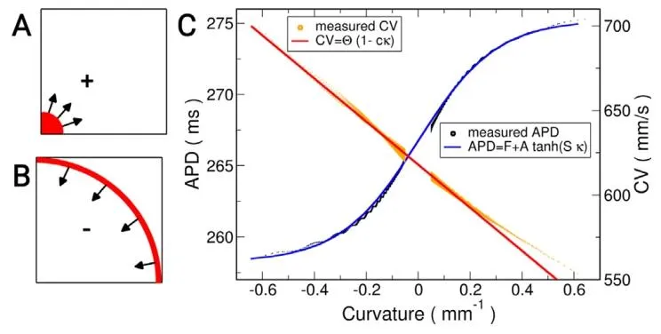
Fig. 2. CV and APD−60 versus curvature fit. A Schematic of stimulation region(red) to initiate positive curvature wavefront. B Schematic of stimulationregion (red) to initiate negative curvature wavefront. C Simulated data pointswere fit by the indicated functions for the CV and APD−60 of the Courtemanchehuman atrial ionic model (Courtemanche et al., 1998).
图2 传导速度(CV)与动作电位时程(APD₋₆₀)随曲率变化的拟合结果 A:用于启动正曲率波前的刺激区域示意图(红色标注)。 B:用于启动负曲率波前的刺激区域示意图(红色标注)。 C:针对Courtemanche人心房离子模型(Courtemanche等,1998),采用指定函数对传导速度(CV)和动作电位时程(APD₋₆₀)的模拟数据点进行拟合的结果。
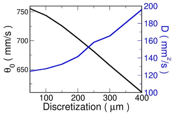
Fig. 3. Effect of discretization on CV and diffusion coefficient, 𝐷, for TT2ionic model. CV (black line) decreases as the element edge length is increased,while the measured diffusion coefficient (blue line) increases. The theoreticaldiffusion constant was 143 mm2∕s.
图3 离散化对TT2离子模型传导速度(CV)与扩散系数(D)的影响 黑色曲线代表传导速度(CV),随单元边长增加而降低;蓝色曲线代表实测扩散系数(D),随单元边长增加而升高。该模型的理论扩散系数为143 mm²/s。
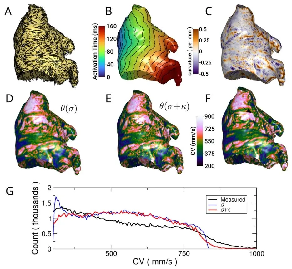
Fig. 4. Conduction velocity in an anisotropic left atrial model. A: Anteroposterior view of fibre orientation. B: Activation pattern with isochrones spaced every10 ms shown. C: Anisotropic curvature computed from activation pattern in (B). D: Conduction velocity based only on conductivity and propagation direction. E:Conduction velocity based on (D) and curvature. F: Measured conduction velocity. G: Histograms of conduction velocity distributions. The measured distribution(black) is compared to those computed only considering the wavefront normal and fibre orientation (blue), and additionally using curvature (red).
图4 各向异性左心房模型中的传导速度 A:心肌纤维方向的前后视图。 B:激动模式图,等时线间隔为10 ms。 C:根据(B)中的激动模式计算得到的各向异性曲率。 D:仅基于电导率与传导方向的传导速度。 E:结合(D)与曲率计算得到的传导速度。 F:实测传导速度。 G:传导速度分布直方图。黑色曲线代表实测分布,蓝色曲线代表仅考虑波前法线与纤维方向的计算分布,红色曲线代表额外结合曲率的计算分布。

Fig. 5. Recovery of 𝜃0 . Histogram of CVs after correcting for conductivity(black), and conductivity and curvature (red). The velocity of a plane wave inthe longitudinal direction, 𝜃0 , was 840 mm/s (green). Bins are 5 ms wide.
图5 固有传导速度(θ₀)的恢复结果 黑色直方图代表仅校正电导率后的传导速度(CV)分布,红色直方图代表校正电导率与曲率后的传导速度分布。纵向方向平面波的速度(即固有传导速度θ₀)为840 mm/s(绿色标注)。直方图的区间宽度为5 ms。

Fig. 6. Components of curvature. The total curvature (anisotropic) is broken down into the geometrical component determined strictly by the wavefront, and amaterial curvature, based on the fibre field. The green arrow indicates the stimulation site, while the red arrow indicates a wavefront collision. Isochrones spacedevery 10 ms are displayed on each surface.
图6 曲率的构成成分 各向异性总曲率可分解为两部分:一是仅由波前决定的几何曲率成分,二是基于纤维场得到的材料曲率成分。 绿色箭头标注刺激位点,红色箭头标注波前碰撞位点。每个表面上均显示了间隔为10 ms的等时线。
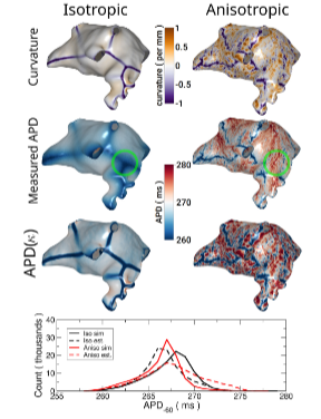
Fig. 7. Effect of curvature on Action Potential Duration (APD) in a left atrialmodel. The left column shows isotropic propagation while the right columnshow anisotropic propagation. Top row: curvature. Same data as in Fig. 4 butopposite view. Second row: measured APD−60. The green circle highlights aregion of large curvature discrepancy due to anisotropy. Third row: APD−60estimated from curvature. Bottom: Histogram of APDs at model nodes for thefour cases shown.
图7 左心房模型中曲率对动作电位时程(APD)的影响 左列展示各向同性传导情况,右列展示各向异性传导情况。 首行:曲率分布,数据与图4一致,但视角相反。 第二行:实测动作电位时程(APD₋₆₀),绿色圆圈标注因各向异性导致曲率存在显著差异的区域。 第三行:基于曲率估算得到的动作电位时程(APD₋₆₀)。 末行:上述四种情况(各向同性/各向异性传导下的实测与估算APD)对应的模型节点APD分布直方图。

Fig. 8. Left apex pacing in lapine left ventricle. A: activation times and curvature B: Measured APD (left) and APD calculated from curvature (right). C: Conductionvelocity computed only from wavefront conductivity, 𝜎 (top), wavefront conductivity and curvature, 𝜎 and 𝜅 (middle), and measured from simulation (bottom).D: Histograms of CVs for the three cases in C with 5 ms bins.
图8 兔左心室心尖部起搏实验结果 A:激动时间与曲率分布。 B:左侧为实测动作电位时程(APD),右侧为基于曲率计算得到的动作电位时程(APD)。 C:上方为仅通过波前电导率(σ)计算的传导速度(CV),中间为结合波前电导率(σ)与曲率(κ)计算的传导速度(CV),下方为模拟实验中实测的传导速度(CV)。 D:对应C中三种情况的传导速度(CV)分布直方图,区间宽度为5 ms。
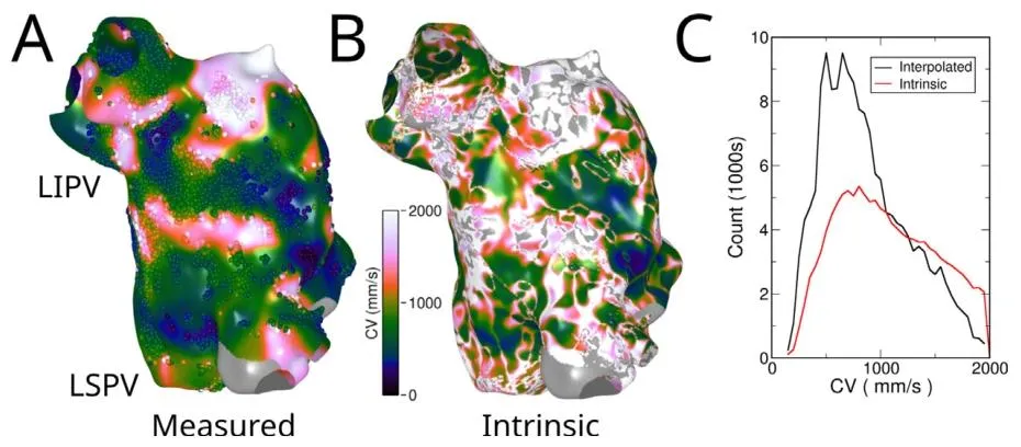
Fig. 9. Estimation of intrinsic left atrial CV. A: Clinically acquired CV data from electroanatomic mapping system projected on to a finer mesh. Grey indicatesmissing data. Dots indicate measured points. B: Reconstructed intrinsic CV taking into account conductivity and curvature. Grey indicates missing data and dataclearly out of physiological range (𝐶𝑉 < 0 or 𝐶𝑉 > 2000 mm∕s. C Histogram of CVs for map in A (interpolated) and B (intrinsic). LSPV: left superior pulmonaryvein, LIPV: left inferior pulmonary vein.
图9 左心房固有传导速度(CV)的估算结果 A:从电解剖标测系统获取的临床传导速度(CV)数据,投影至更精细的网格上。灰色区域代表缺失数据,圆点代表实测数据点。 B:结合电导率与曲率重建得到的固有传导速度(CV)。灰色区域代表缺失数据及明显超出生理范围(CV<0或CV>2000 mm/s)的数据。 C:传导速度(CV)分布直方图,分别对应A图(插值后的临床数据)与B图(固有CV数据)。图中LSPV指左上肺静脉,LIPV指左下肺静脉。
Table
表
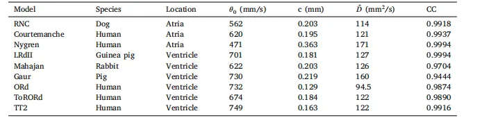
Table 1Conduction velocity dependency on curvature. Simulated CV was fit with function of the form 𝜃(𝜅) = 𝜃0 (1 − 𝑐𝜅)where 𝜅 is the curvature (mm−1), 𝜃0 is the CV at zero curvature, 𝑐 is the sensitivity to curvature, and the computeddiffusion coefficient ̃𝐷* which theoretically has the value of 143 mm2/s. The correlation coefficient (CC) of thefit is given.
表1 传导速度(CV)对曲率的依赖性 模拟得到的传导速度(CV)采用如下形式的函数拟合:θ(κ) = θ₀(1 − cκ)。 其中,κ为曲率(单位:mm⁻¹),θ₀为曲率为零时的传导速度(CV),c为对曲率的敏感度,D̃为计算得到的扩散系数(理论值应为143 mm²/s)。表中同时给出了拟合的相关系数(CC)。
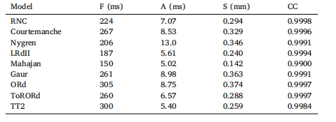
Table 2Action Potential Duration (APD) dependency on curvature when fit withfunction of the form 𝐴𝑃 𝐷−60(𝜅) = 𝐹 + 𝐴 tanh (𝑆𝜅) where 𝜅 is the curvature(mm−1), 𝐹 is the APD at zero curvature, 𝐴 is the range of APD change, and𝑆* is the sensitivity to curvature. The correlation coefficient (CC) of the fit isgiven.
表2 动作电位时程(APD)对曲率的依赖性 动作电位时程(APD)采用如下形式的函数拟合:APD₋₆₀(κ) = F + A tanh(Sκ)。 其中,κ为曲率(单位:mm⁻¹),F为曲率为零时的动作电位时程(APD),A为APD的变化范围,S为对曲率的敏感度。表中同时给出了拟合的相关系数(CC)。